
DataScience Workbook / 07. Data Acquisition and Wrangling / 3. Data Wrangling: ready-made apps / 3.3 Split data or create data chunks (python)
Introduction
The bin_data.py ⤴ application is written in Python3 and employs efficient libraries [pandas and numpy] for operating on a complex data structure. The application aggregates observables [by summing or averaging numerical values] over the data slices (rows grouped in a slice). The statistic (STATS) is calculated separately for each column of numerical values, while R = ‘ranges-column’ can be used to bin data based on the incrementation of values.
Aggregating observables facilitates:
- coarsening the patterns of observed feature
- detecting regions/ranges enriched or depleted by the feature
- assessing the significance threshold of measured feature
Algorithm
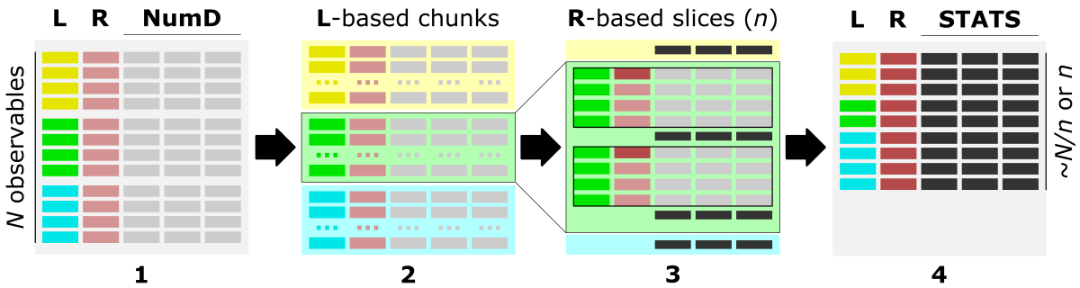
The figure shows the main steps of the bin_data algorithm.
1) The optimal data structure requires:
L - label-column, a column of labels,
R - ranges-column, numerical [int, float] column of data characteristic (index, position, increment, feature),
numD - data-columns, any number of numerical columns that will be aggregated.
2) First, data is split into chunks based on assigned category labels (L). Optionally, sing -s 'true' option, chunks can be saved into separate CSV files, which facilitates Big Data loading in the repetitive analyses.
3) Next, each L-based data chunk is split into slices composed of a specific number of consecutive rows, typically based on the R column.
The type of slices can be requested using the -t option as:
- steps, where the size of the slice is user-provided as the number of consecutive data rows (n); the returned output contains
~N/nslices (where N is the number of rows in the input file); rows count in each slice is the same; - bins, where the number of slices is user-provided (n); the returned output contains
nslices; rows count in each slice is the same; - value, where the slices are cut based on the increment of the value in the selected (numerical) R column (use the
-roption to specify the'ranges-column'index); the returned output may contain a different number of slices (bins) depending on the coarseness of the value increment (n, [int or float]); rows count in each slice can be different, so the additional column'counts'is added into the output to facilitate tracking of empty bins;
The slicing procedure is performed separately for each category (if multiple are provided) stored in the L = ‘labels-column’, use the -l option. If the user is interested in processing selected labels only, they can be inputed with the -ll option as a one-column file or inline comma-separated string.
4) Data stored in each numerical column (NumD) is aggregated over the rows in a given slice. So, the single row of data per slice is returned in the output.
The user choose to sum or average values in the numerical columns as the calculated statistics (STATS) with the option -c followed by string argument 'sum' or 'ave', respectively.
In the output, the R = ‘ranges-column’ (with the default ‘position’ header) stores starting position in the slice or range of incremented values.
Requirements
Requirements: python3, pandas, numpy
Install Python3 on various operating systems (if you don't have it yet)
sudo apt-get update
sudo apt-get install python3
if not yet, first install Homebrew:
/bin/bash -c "$(curl -fsSL https://raw.githubusercontent.com/Homebrew/install/HEAD/install.sh)"
brew install python3
Please follow the instructions provided at phoenixnap.com .
Install app requirements
pip3 install pandas
pip3 install numpy
Options
help & info arguments:
  -h,         --help                    # show full help message and exit
  -v level,   --verbose level           # [int] increase verbosity: 0 = warnings, 1 = info, 2 = rich info
required arguments:
-i input,     --data-source input       # [string] input multi-col file or directory with data chunks
-l label,     --labels-col label        # [int]    index of column with labels used to chunk data
-r range,     --ranges-col range        # [int]    index of column with ranges used to slice data
optional arguments:
  -ll llist,  --label-list llist        # [path] or [comma-separated list] provide custom list of labels to be processed
  -hd header, --header header           # [list]            provide custom ordered list of columns names (header)
  -ch chunks, --chunk-size chunks       # [int]             provide custom size of chunks (number of rows loaded at once)
  -s save,    --chunk-save save         # {true,false}      saves data into chunked files
  -c calc,    --calc-stats calc         # {ave,sum}         select resizing operation: ave (mean) or sum
  -t type,    --slice-type type         # {step,bin,value}  select type of slicing: 'step' (number of rows in a slice) or 'bin' (number of slices) or 'value' (value increment in ranges-col)
  -n slice,   --slice-size slice        # [float]           select size/increment of slicing
  -d dec,     --decimal-out dec         # [int]             provide decimal places for numerical outputs
  -o out,     --output out              # [string]          provide custom output filename
defaults for optional arguments:
-ll None                # means: all labels will be processed
-hd None                # means: assigning 'label' for labels-col, 'position' for ranges-col, and 'val-X' for remaining columns, where X is an increasing int number
-ch None                # means: optimizing number of loaded input rows for 250MB memory usage
-s 'true'               # means: data chunked by unique labels will be saved in CSV format into the CHUNKS/ directory; disabled when input is a directory
-c 'ave'                # means: average of each numerical column in the slice will be returned
-t 'step'               # means: data will be sliced by the number of rows in a slice (each slice consists of the same number of rows)
-n 100                  # means: (-t 'step') the slice will be composed of 100 rows or (-t 'bin') there will be 100 slices in total or (-t 'value') the increment for slicing will be 100
-d 2                    # means: 2 decimal places will be kept for all numeric columns
-o 'output_data'        # means: the output will be saved as 'output_data.csv' file
Usage (generic)
syntax:
^ arguments provided in square brackets [] are optional
python3 bin_data.py -i input -l label -r range [-ll labels_list] [-hd header_names]
                   [-ch chunks_size] [-s {true,false}]
                   [-c {ave,sum}] [-t {step,bin,value}] [-n slice]
                   [-d dec] [-o out]
                   [-v [VERBOSE]] [-h]
^ arguments provided in square brackets [] are optional
example usage with minimal required options:
python3 bin_data.py -i input_file -l 0 -r 1
The example parses the single text-like input_file, where the L = ‘label-column’ has index 0, and R = ‘ranges-column’ has index 1.
Hands-on tutorial
Environment setup
The application is developed in Python programming language and requires importing several useful libraries. Thus, to manage dependencies, first you have to set up the Conda environment on your (local or remote) machine.
- When you don’t have Conda yet…
To install Conda ⤴ environment management system and configure an instance for data wrangling applications, follow a step-by-step instructions provided in the tutorial Data Wrangling: Environment setup ⤴.
- Once you have Conda and the data_wrangling environment follow further steps below
Activate existing Conda environment
You do NOT need to create the new environment each time you want to use it. Once created, the env is added to the list of all virtual instances managed by Conda. You can display them with the command:
conda info -e
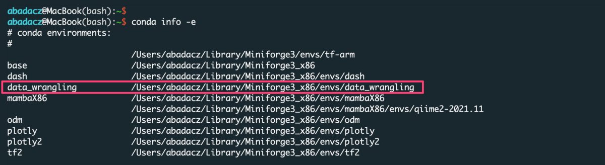
The selected environment can be activated with the conda activate command, followed by the name of the env:
conda activate data_wrangling

Once the environment is active, you can see its name preceding the prompt.
Install new dependencies within environment
Once environment of your choice is activated, you can install new dependencies required by the selected application.
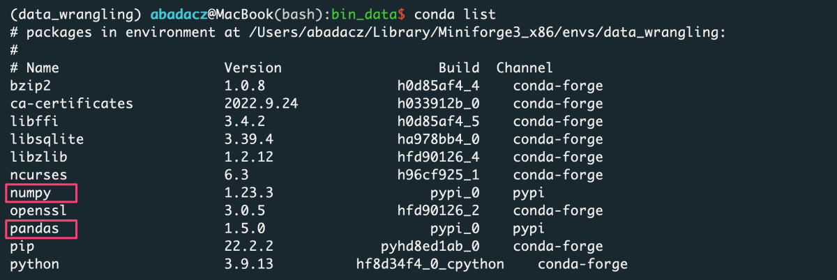
The bin_data ⤴ application requires:
- pandas ⤴, to create and manage data structure
- numpy ⤴, to manipulate advanced numerical data structures
Generally, you can try to install modules with the conda install {module=version} command. However, since we initialized the data_wrangling environment with Python=3.9, we can also install modules using pip install {module==version}, as follows:
pip install pandas
pip install numpy
Note that if you do not indicate the version of the module you are installing, the latest stable release will usually be installed.
When you install by
conda, assign the module's version using a single equals sign =. When you install by
pip, assign the module's version using a double equals sign ==.
If you don't know whether a particular library is already installed in your Conda environment, you can check it using the
conda list command. Your terminal screen will display a list of installed software in the active environment.
Inputs
Before using the application, make sure your inputs has been properly prepared. First of all, the data in the input file must be organized into columns. The number of columns and rows is arbitrary, including Big Data support.
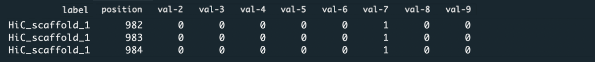
data structure in the example input.txt
HiC_scaffold_1  982     0       0       0       0       0       1       0       0
HiC_scaffold_1  983     0       0       0       0       0       1       0       0
HiC_scaffold_1  984     0       0       0       0       0       1       0       0
HiC_scaffold_1  985     0       0       0       0       0       1       0       0
HiC_scaffold_1  986     0       0       0       0       0       1       0       0
HiC_scaffold_1  987     0       0       0       0       0       1       0       0
...
HiC_scaffold_10 547     3       1       0       0       1       0       0       0
HiC_scaffold_10 548     3       1       0       0       1       0       0       0
HiC_scaffold_10 549     3       1       0       0       1       0       0       0
HiC_scaffold_10 550     3       1       0       0       1       0       0       0
File format
The format of the input file does NOT matter as long as it is a columns-like text file. Text (.txt) files with columns separated by a uniform white character (single space, tabulator) or comma-delimited CSV files are preferred, though.
Data delimiter
The data delimiter used does NOT matter, as it will be automatically detected by application. However, it is essential that the column separator is consistent, for example, that it is always a fixed number of spaces ` only or always a tab, \t. If separator is a comma ,` remember NOT to use it inside a given data cell (e.g., if the values in the column are a list).
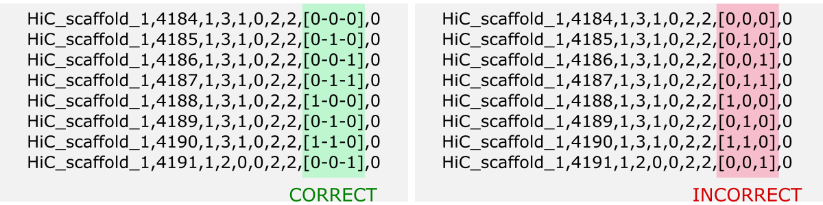
Note that only data from numeric columns will be aggregated. So, if the values in a column are a list, so even if the values in the list are numeric, such a column will be treated as a string.
If you want to process such data, change the data structure of the input so that the values in the list split into separate columns.
Column names
The header is usually the first line of the file and contains the column labels. Naming the columns brings great informational value to the analyzed data. However, the application does NOT require the input file to have a header. If it is in the file it will be detected automatically. Otherwise, the default set of column labels [ see options section ] will be assigned.
File content
Running the application requires that you specify the index of the labels and ranges columns.
Labels column should contain labels or categories assigned to the observables. They are used to aggregate values over data chunks corresponding to the unique labels. The values in the labels column can be strings or numerical.
If all your data belong to the same or none category, you can add to your file a fake-label column with all identical values, e.g., ‘label’ or 0.
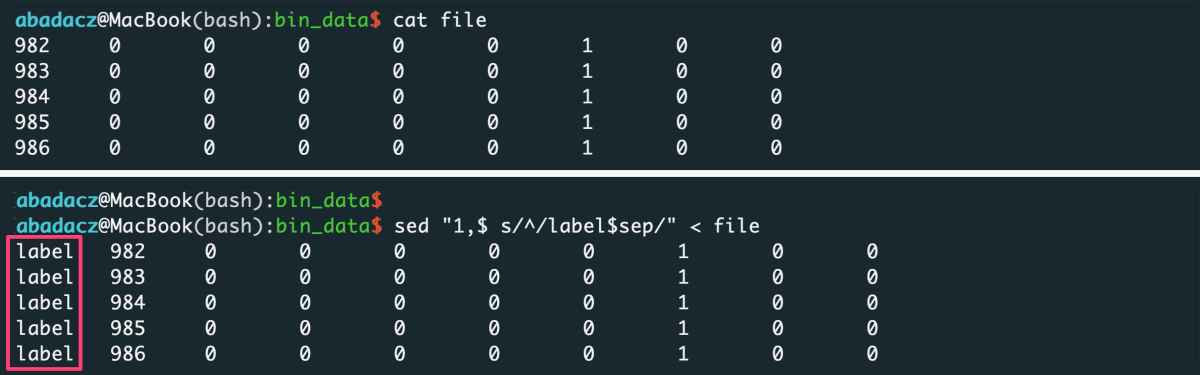
- input file without header
sep='\t'
sed "1,$ s/^/value$sep/" < file > input
^ paste your separator within ‘ ‘ of $sep variable
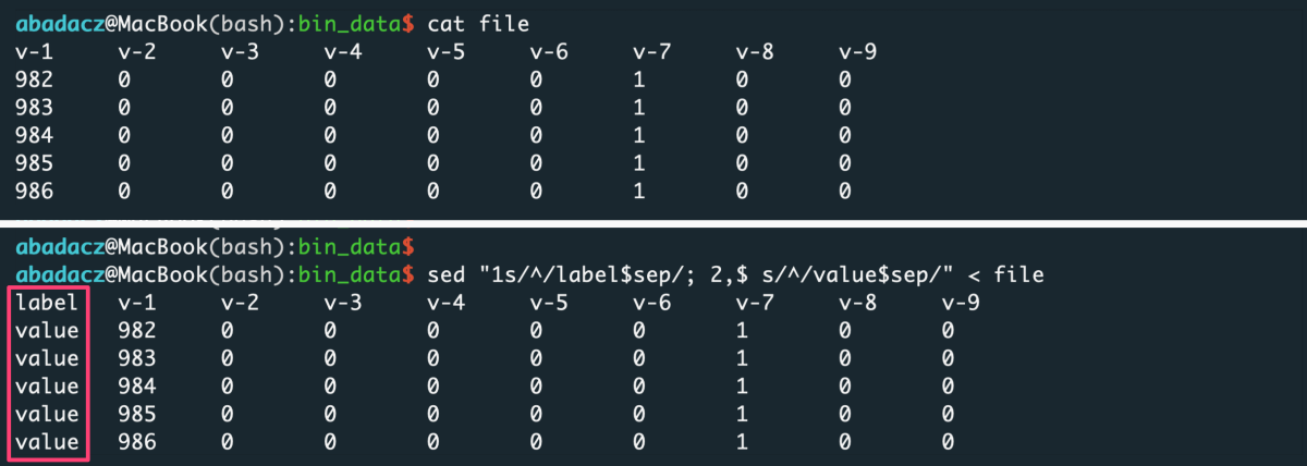
- input file with header
sep='\t'
sed "1s/^/label$sep/; 2,$ s/^/value$sep/" < file > input
^ paste your separator within ‘ ‘ of $sep variable
Ranges column, in general, should contain numerical values used to determine ranges for data slicing.
The application provides the ability to slice data by three different scenarios:
step, with constant number of rows in a slicebin, with constant number of slicesvalue, with constant increment of values in ranges col
After data aggregation over each slice, the numerical values from the ranges-col [R] will be concatenated to the single value defined as a range from-to [R’] (see figure below).
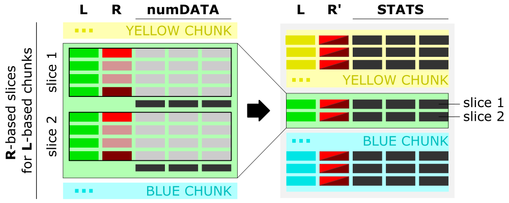
The figure shows the algorithm of data aggregation over the slice. The detailed description is provided in the next paragraph.
Interpretation of ranges column [R]
- The input is grouped into the data chunks corresponding to unique categories/labels [L, left panel], here marked in yellow, green, and blue. Each chunk is further split into slices based on user-selected slicing
typeandrange. The figure shows sample slices of the green chunk. - For each slice, the data from all numerical columns [numDATA, left panel] is aggregated to a single value per column and represents
sumormean. These values correspond to STATS columns on the right panel. - The first and the last value in the ranges column [R, left panel] for each slice creates a tuple saved in the ranges column [R’, right panel] of the aggregated data row in the output.
Contents of range column vs. type of slicing
- constant row counts per slice
Generally, when you want to slice the data with an equal number of rows, you should use step (user-provided number of rows per slice) or bin (user-provided number of slices) type of slicing. In this case, only first and last value from the ranges column will be reported for the aggregated output row of a data slice. Thus, data in labels-based chunks will be initially sorted by values in the ranges column.
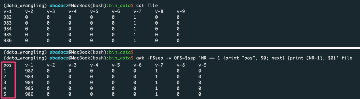
If you want to keep the original ordering of an input, add a column with generic indexing and pass this column index with the -r option:
sep='\t'
awk -F$sep -v OFS=$sep 'NR == 1 {print "position", $0; next} {print (NR-1), $0}' file > input
^ paste your separator within ‘ ‘ of $sep variable
- variable row counts per slice
e.g., when the number of observations changes for a value increment of a selected feature
Generally, when you want to slice the data based on the value increment of a selected feature (i.e., bin the observations due to the constant-length ranges of the feature values), you should use a value type of slicing. Also, you should indicate the index of that feature column as the ranges column (with the -r option) and pass the value increment with option -n.
In this case, the first value from the ranges column and the first + increment will be reported for the aggregated output row of a data slice.
Usage variations
Create label-based data chunks
Use this example to split data stored in a single file by categories assigned to every row. For each label a separate file will be created and all files will be saved in the CHUNKS directory on the current path. You can use Bash scripting to split small data, however, for large datasets (GBs of text file size) this python application will be significantly more efficient.
Input
The input can be a text file with any number of data columns of any type (strings or numerical).
File Preview below - Download full example input.txt Download ⤵
      0	1	2	3	4	5	6	7	8	9
---------------------------------------------------------
label_1	982	0	0	0	0	0	1	0	0
label_1	983	0	0	0	0	0	1	0	0
label_1	984	0	0	0	0	0	1	0	0
label_1	985	0	0	0	0	0	1	0	0
...
label_10	2263	0	0	0	0	0	1	0	0
label_10	2264	0	0	0	0	0	1	0	0
label_10	2265	0	0	0	0	0	1	0	0
You need to select one column used to split data into the categories based on the set of unique values (labels). The label-col can be text or numerical.
App usage
In this example we will use the first column with text-like labels to create data chunks. In Python numbering starts from 0, so the index of the first column is 0. Index of the selected label-col is feed to the algorithm with the option -l.
To exit the algorithm just after splitting the data and saving the chunks, set the ranges-col argument to ‘off’ with the option -r.
python3 bin_data.py -i input.txt -r 'off' -l 0
Output
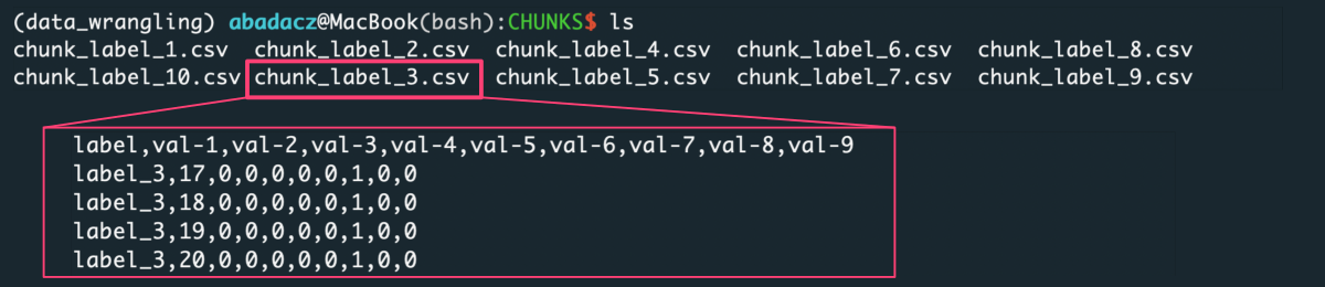
In result, the CHUNKS directory will be crated and within it the number of files corresponding to the set of unique labels will be saved in comma-separated CSV format.
Create data chunks of N rows
Use this example to split data into slices of N rows. For each data chunk a separate file will be created and all files will be saved in the CHUNKS directory on the current path. You can use Bash scripting to split small data, however, for large datasets (GBs of text file size) this python application will be significantly more efficient.
Input
The input can be a text file with any number of data columns of any type (strings or numerical).
File Preview below - Download full example input.txt Download ⤵
      0	1	2	3	4	5	6	7	8	9
---------------------------------------------------------
label_1	982	0	0	0	0	0	1	0	0
label_1	983	0	0	0	0	0	1	0	0
...
label_10	2264	0	0	0	0	0	1	0	0
label_10	2265	0	0	0	0	0	1	0	0
You need to specify the number of rows, N, that will create a single data chunk.
App usage
In this example we will split data by every 100 rows that requires using the -n 100 -t 'step' options. Each dat chunk will contain a 100 consecutive rows regardless of assigned labels (if any) so the -l must be ‘off’.
To exit the algorithm just after splitting the data and saving the chunks, set the ranges-col argument to ‘off’ with the option -r.
python3 bin_data.py -i input.txt -r 'off' -l 'off' -n 100 -t 'step'
Output
In result, the CHUNKS directory will be crated and within it the number of 100-rows files will be saved in comma-separated CSV format.
Create N equal data chunks
python3 bin_data.py -i input.txt -r '' -l '' -n 10 -t 'bin'
Input file vs. Input directory
python3 bin_data.py -i hybrid.depth -l 0 -r 1 -t 'step' -n 1000 -s True -v 1
python3 bin_data.py -i CHUNKS/ -l 0 -r 1 -t 'value' -n 0.15 -s 'false' -v 0
Aggregate data over every N rows
python3 bin_data.py -i input.txt -l 0 -r 1 -t 'step' -n 100 -s True -v 1
Aggregate data over each of N slices
python3 bin_data.py -i input.txt -l 0 -r 1 -t 'bin' -n 10 -s True -v 1
Aggregate data over value increment
python3 bin_data.py -i input.txt -l 0 -r 1 -t 'value' -n 0.1 -d 3 -s True -v 1