Introduction
Excel is most popular among researchers because of its ease of use and tons of useful features. In most cases scripting is the most efficient way to do these simple operations, but practicality of Excel for researchers and the cryptic scripting commands will always make excel a better choice.
TASK or CHALLENGE
If you require two spreadsheets to merge based on a shared column, this tutorial will guide you through automating the process, making it more efficient and minimizing the risk of errors.
Merge two spreadsheets using a common column
Combining data from two spreadsheets based on a common column can be a complex and time-consuming task, especially when dealing with large datasets. Manually merging data can be tedious and prone to errors. This tutorial provides a step-by-step guide to automate the merging process using the bioinformatics dataset as an example.
In Bioinformatics, most common case of merging 2 spreadsheets is when users have a list of gene ids and another list of gene ids with function. To merge these 2 sheets by the gene ids, we can use the VLOOKUP function in Excel.
By the end of this tutorial, you will be able to efficiently merge two spreadsheets in Excel using a common column, ensuring accurate and streamlined data integration.
Data
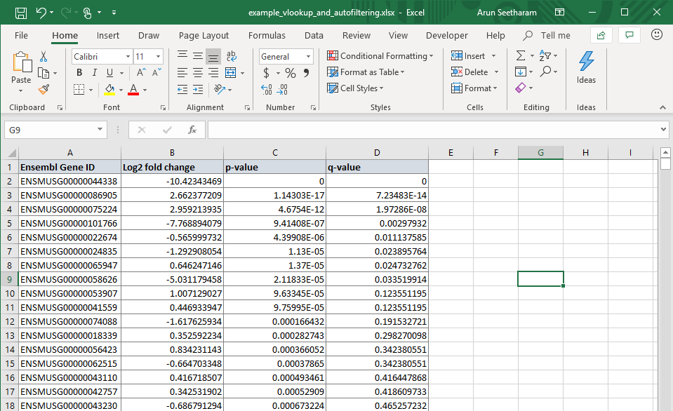
Typically, users will have something like this:
Sheet1 : list of gene ids with differential gene expression results
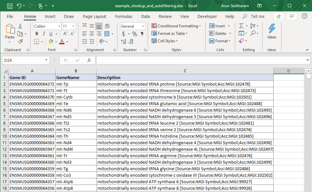
Sheet2: list of gene ids with its annotation information
You can use any Excel file that contains at least 2 spreadsheets with a common column to complete this exercise. Or, you can simply an example Excel file used in this demonstartion.
You should get an Excel file with 2 worksheets. Each worksheet may contain different number of rows. This is just a fragment of the original dataset.
Now, the task is to add GeneName and Description (i.e., Function) information for the Sheet1 using the information from Sheet2 with the Ensembl Gene ID and Gene ID as the common field/column. We can use the VLOOKUP function to complete this task.
Excel Formula
Type =VLOOKUP on the Sheet1 in an empty E1 cell. You should see typical usage for the command as shown below.
It needs 4 pieces of information:
| parameter | description | explanation |
|---|---|---|
lookup_value |
Which cell to use for looking up the value? | Since we need to look up information for Ensembl Gene ID in Sheet1, it should be A2 cell here. |
table_array |
Where to look up? | The entire table where the annotation is stored. This should be the full table in Sheet2 (in this case: Sheet2!$A$2:$C$49672). |
col_index_num |
What cell value to print for matching ids? | Since we need Gene Name and it is the 2nd column of Sheet2, we should use the value of 2 here. |
range_lookup |
Do you need an exact match or approximate match? | Since each gene id is unique, we need exact match, so we fill FALSE here. |
The complete formula looks like this:
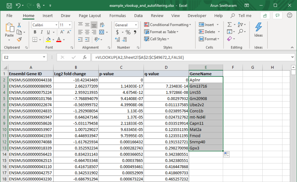
=VLOOKUP($A2,Sheet2!$A$2:$C$49672,2,FALSE)

Note the $ syntax for rows and/or columns of the parameters lookup_value and table_array, this prevents the Excel from incrementing when the formula is dragged to other cells. This is because we want to keep out the Ensembl Gene ID column and both rows and columns for the table_array fixed, regardless of where we use the formula in the Sheet1.
Next, we need to propagate this formula for all records. You can simply drag this formula down using the + sign that appears on the lower right of the cell containing formula. You can also double click on it to automatically fill the formula for you. It should correctly fill in the GeneName column for you.
For filling out the Function follow the same steps, but instead of using col_index_num value of 2, we will use 3 which corresponds to Description in the Sheet2.
=VLOOKUP(A2,Sheet2!$A$2:$C$49672,3,FALSE)
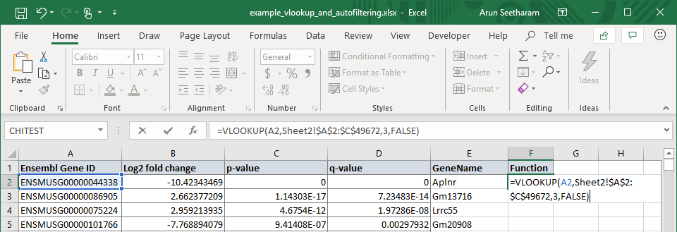
Again, click and drag or double click the + sign that appears on the lower right of the cell to fill all other cells in that column.
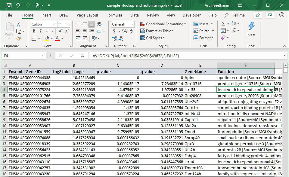
You should now have the complete information in a single table with both functions and gene names assigned to Gene ID!
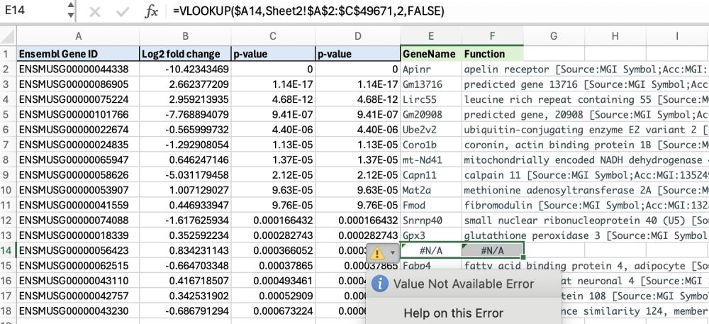
Merging data using a shared column is also a good way to check the completeness of the dataset. This approach makes it easy to detect records with missing information, as the transferred cells with missing data will be marked as #N/A or display an error.
