
DataScience Workbook / 08. Data Visualization / 2. Introduction to Scientific Graphing / 2.3 RStudio – Data Processing & Plotting with R / Creating Heatmaps in R using ComplexHeatmap
Introduction
ComplexHeatmap in R
The GitHub repo ⤴ and the complete reference guide ⤴ for the ComplexHeatmap package is available.
The complete reference document contains all the details about this package but can be overwhelming due to the amount of information. The following tutorial should get you started on using ComplexHeatmap by making simple heatmap and adding some features to it. Check out the Intro to R ⤴ page to get started in learning R programming.
Installation
ComplexHeatmap package needs to be installed and loaded:
install.packages("BiocManager")
BiocManager::install("ComplexHeatmap")

# Load package
library(ComplexHeatmap)  # directly load the package if it is installed already
Load dataset
Your dataset needs to be loaded in the form of a matrix.
# Loaded the dataset in matrix named mat
mat <- as.matrix(read.csv ("PATH/TO/file.csv", sep = ',', row.names = 1, header=T))
# Other file formats can also be loaded as matrix
# mat[1:5,1:3]   #to view the matrix
If the dataset has non-numeric entries, the matrix might be loaded as character type and can lead to heatmap not displaying properly. If this is a problem, get rid of the non-numeric characters and convert the matrix type to numeric (see below).
According to the complete reference documentation: "NA is allowed in the matrix. You can control the color of NA by na_col argument (by default it is grey for NA). A matrix that contains NA can be clustered by Heatmap() as long as there is no NA distances between any of the rows or columns respectively."
# after loading the data as.matrix, check matrix type in the environment panel in RStudio or by using:
typeof(mat)
# If matrix type is character,  it returns "character". You need to replace any characters with numbers.

mat[mat == "None"] <- 0    # replaces the word "None" anywhere in mat with 0

# Once the matrix contains only numerals, change it's type:
mat <- type.convert(mat, as.is = TRUE)

Now, typeof(mat) returns "double" then matrix is numeric. You can also use
is.numeric(mat)
which should return TRUE
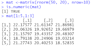
For this tutorial, I will make a random matrix to use as an example.
# Generate random matrix
mat <- matrix(rnorm(50, 20), nrow=10)
is.numeric(mat) # check if numeric
mat[1:5,1:3] # view selected rows and columns
# The output is shown below
Generate simple heatmap
This command generates a heatmap with default settings without additional commands:
Heatmap(mat) # mat is the dataset name loaded earlier as matrix
The commands in R are case sensitive, so heatmap and Heatmap are commands from two different packages.
Customize your heatmap
There are countless ways to customize your heatmap with R. Here are a few of the ways to make a great heatmap.
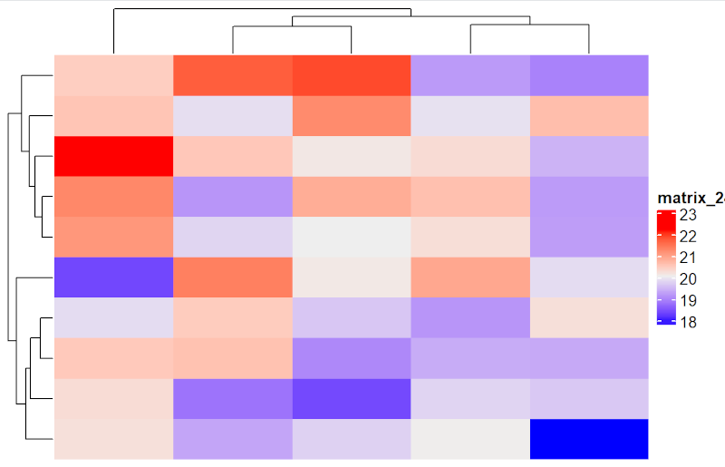
Select different colors
Use RColorBrewer package to get a variety of color palettes. Always select colorblind accessible color combinations. You can input colors using palettes directly from RColorBrewer or using the hex codes to specify exact hues.
library(RColorBrewer)
library(circlize)

display.brewer.all(colorblindFriendly=TRUE)

# col_fun <- colorRamp2(c(18, 20, 23), brewer.pal(3, "Blues"))
# OR
col_fun <- colorRamp2(c(18, 20, 23), c("#FFFFB2", "#f4a582", "#BD0026"))
# The `colorRamp2` function is used for color interpolation.

Heatmap(mat, name = "mat", col = col_fun)
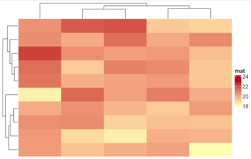
Draw heatmap with custom labels on legend
Heatmap(mat,
        heatmap_legend_param = list(
          title = "Legend title", at = c(18, 20, 23),
          labels = c("label1", "2", "three")
        )
)
# Numbers in parameter at=c() appear on legend unless labels=c() is included.
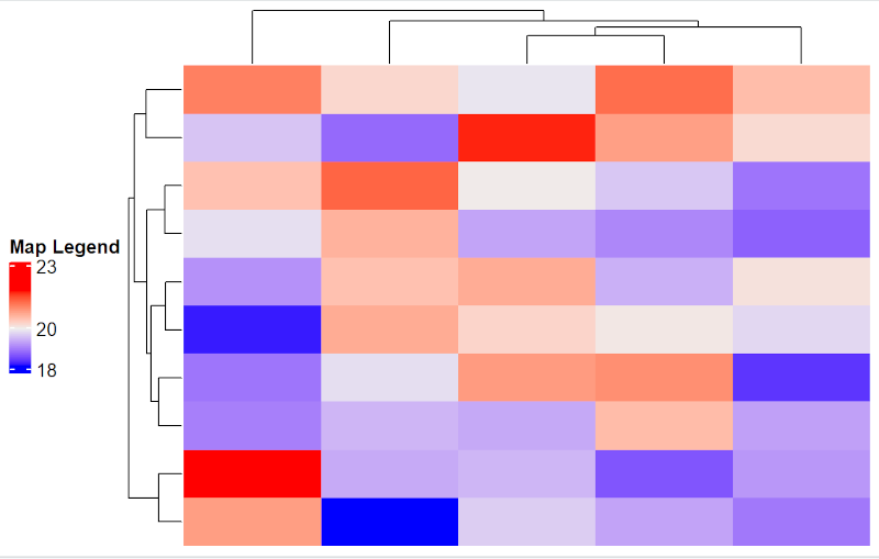
Customize legend
You can specify title, annotation, and position of legend.
Legend_details <- list(title = "Map Legend",
                       at = c(18, 20, 23)
)
map1 <- Heatmap(mat, heatmap_legend_param = Legend_details)
draw(map1, heatmap_legend_side = "left")   # Can be “right”, “left”, “bottom”, “top”
Draw independent legend for more flexibility
Note that this legend is independent of the plot, so you need to select the same colors carefully for representing the corresponding plot.
col_fun <- colorRamp2(c(18, 20, 23),
                      c("#d1e5f0", "#f4a582", "#d6604d"))
# create a function to represent color, which can be used for both legend and heatmap to avoid selecting different colors for both

grid.newpage()
lgd = Legend(col_fun = col_fun, title = "Legend title")
lgd1 = draw(lgd, x= unit(0.9, "npc"), y=unit(0.2, "npc"))

The numbers 0.9 and 0.2 in the last line of code represent the position of legend on x and y axis of the entire plot and can be changed according to your need. This gives you more flexibility with the positioning of the legend.
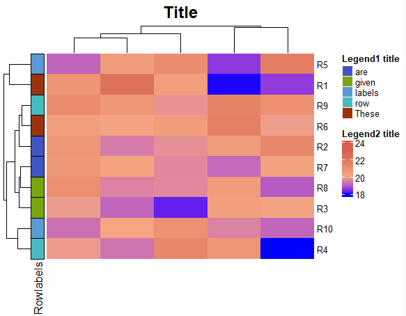
Add more annotations to the plot
ComplexHeatmap package allows you to modify the plot in lots of ways. Here is an example of a complex heatmap with additional annotations.
mat <- matrix(rnorm(50, 20), nrow=10)
rownames(mat) = paste0("R", 1:10)
labels <- data.frame(Rowlabels = c("These", "are", "given", "row", "labels", "These", "are", "given", "row", "labels"))

### Define annotations

ha_row = rowAnnotation(df= labels,
                       gp = gpar(col = "black"),
                       annotation_legend_param = list(title = "Legend1 title",
                                                      ncol = 1)
                       )

col_fun <- colorRamp2(c(18, 20, 23),
                      c("Blue", "#f4a582", "#d6604d"))

### Make the heatmap
map <- Heatmap(mat, show_heatmap_legend = TRUE, col=col_fun,
               heatmap_legend_param = list(title = "Legend2 title", ncol = 1),
               column_title = "Title",
               left_annotation = ha_row,
               column_title_gp = gpar(fontsize = 18, fontface = "bold"),
               row_names_gp = grid::gpar(fontsize = 10)
)


draw(map, align_heatmap_legend = "heatmap_top", merge_legends = TRUE)
There are lots of additional features in this package like drawing histograms, boxplots, and violin plots around the heatmap. Check out the complete reference documentation ⤴ for more information.