DataScience Workbook / 08. Data Visualization / 2. Introduction to Scientific Graphing / 2.3 RStudio – Data Processing & Plotting with R

Introduction

Predicting the age of abalone from physical measurements.
Dataset characteristics: multivariate
Attribute type: categorical, integer, real
Subject area: life
Instances: 4177
Associated Tasks: classification
Attributes: 8

abalone <- readr::read_csv( "abalone.data", col_names = F )
names( abalone ) <- c( "Sex", "Length", "Diameter", "Height", "Whole_weight", "Shucked_weight", "Viscera_weight", "Shell_weight", "Rings" )
abalone

## # A tibble: 4,177 × 9
##    Sex   Length Diameter Height Whole_weight Shucked_weight Viscera_weight Shell_weight Rings
##    <chr>  <dbl>    <dbl>  <dbl>        <dbl>          <dbl>          <dbl>        <dbl> <dbl>
##  1 M      0.455    0.365  0.095        0.514         0.224          0.101         0.15     15
##  2 M      0.35     0.265  0.09         0.226         0.0995         0.0485        0.07      7
##  3 F      0.53     0.42   0.135        0.677         0.256          0.142         0.21      9
##  4 M      0.44     0.365  0.125        0.516         0.216          0.114         0.155    10
##  5 I      0.33     0.255  0.08         0.205         0.0895         0.0395        0.055     7
##  6 I      0.425    0.3    0.095        0.352         0.141          0.0775        0.12      8
##  7 F      0.53     0.415  0.15         0.778         0.237          0.142         0.33     20
##  8 F      0.545    0.425  0.125        0.768         0.294          0.150         0.26     16
##  9 M      0.475    0.37   0.125        0.509         0.216          0.112         0.165     9
## 10 F      0.55     0.44   0.15         0.894         0.314          0.151         0.32     19
## # ℹ 4,167 more rows

glimpse( abalone )

## Rows: 4,177
## Columns: 9
## $ Sex            <chr> "M", "M", "F", "M", "I", "I", "F", "F", "M", "F", "F", "M", "M", "F", "F", "M", "I", "F", "M", "M", "M", "I"…
## $ Length         <dbl> 0.455, 0.350, 0.530, 0.440, 0.330, 0.425, 0.530, 0.545, 0.475, 0.550, 0.525, 0.430, 0.490, 0.535, 0.470, 0.5…
## $ Diameter       <dbl> 0.365, 0.265, 0.420, 0.365, 0.255, 0.300, 0.415, 0.425, 0.370, 0.440, 0.380, 0.350, 0.380, 0.405, 0.355, 0.4…
## $ Height         <dbl> 0.095, 0.090, 0.135, 0.125, 0.080, 0.095, 0.150, 0.125, 0.125, 0.150, 0.140, 0.110, 0.135, 0.145, 0.100, 0.1…
## $ Whole_weight   <dbl> 0.5140, 0.2255, 0.6770, 0.5160, 0.2050, 0.3515, 0.7775, 0.7680, 0.5095, 0.8945, 0.6065, 0.4060, 0.5415, 0.68…
## $ Shucked_weight <dbl> 0.2245, 0.0995, 0.2565, 0.2155, 0.0895, 0.1410, 0.2370, 0.2940, 0.2165, 0.3145, 0.1940, 0.1675, 0.2175, 0.27…
## $ Viscera_weight <dbl> 0.1010, 0.0485, 0.1415, 0.1140, 0.0395, 0.0775, 0.1415, 0.1495, 0.1125, 0.1510, 0.1475, 0.0810, 0.0950, 0.17…
## $ Shell_weight   <dbl> 0.150, 0.070, 0.210, 0.155, 0.055, 0.120, 0.330, 0.260, 0.165, 0.320, 0.210, 0.135, 0.190, 0.205, 0.185, 0.2…
## $ Rings          <dbl> 15, 7, 9, 10, 7, 8, 20, 16, 9, 19, 14, 10, 11, 10, 10, 12, 7, 10, 7, 9, 11, 10, 12, 9, 10, 11, 11, 12, 15, 1…

abalone %>%
  select( where(is.numeric) ) %>%
  psych::describe() %>%
  kableExtra::kbl() %>%
  kableExtra::kable_styling( bootstrap_options = c("striped", "hover") )

	vars	n	mean	sd	median	trimmed	mad	min	max	range	skew	kurtosis	se
Length	1	4177	0.5239921	0.1200929	0.5450	0.5324783	0.1186080	0.0750	0.8150	0.7400	-0.6394138	0.0616411	0.0018582
Diameter	2	4177	0.4078813	0.0992399	0.4250	0.4146994	0.0963690	0.0550	0.6500	0.5950	-0.6087607	-0.0482711	0.0015355
Height	3	4177	0.1395164	0.0418271	0.1400	0.1402498	0.0370650	0.0000	1.1300	1.1300	3.1265706	75.8953091	0.0006472
Whole_weight	4	4177	0.8287422	0.4903890	0.7995	0.7995646	0.5285469	0.0020	2.8255	2.8235	0.5305773	-0.0264756	0.0075877
Shucked_weight	5	4177	0.3593675	0.2219629	0.3360	0.3439231	0.2349921	0.0010	1.4880	1.4870	0.7185815	0.5912553	0.0034344
Viscera_weight	6	4177	0.1805936	0.1096143	0.1710	0.1733193	0.1178667	0.0005	0.7600	0.7595	0.5914271	0.0809994	0.0016960
Shell_weight	7	4177	0.2388309	0.1392027	0.2340	0.2305173	0.1475187	0.0015	1.0050	1.0035	0.6204809	0.5281636	0.0021538
Rings	8	4177	9.9336845	3.2241690	9.0000	9.6410410	2.9652000	1.0000	29.0000	28.0000	1.1133019	2.3239123	0.0498868

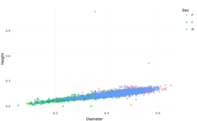
p <- ggplot(abalone, aes(x=Diameter, y=Height, color=Sex)) + geom_point() + theme_minimal()
p <- ggplotly(p)

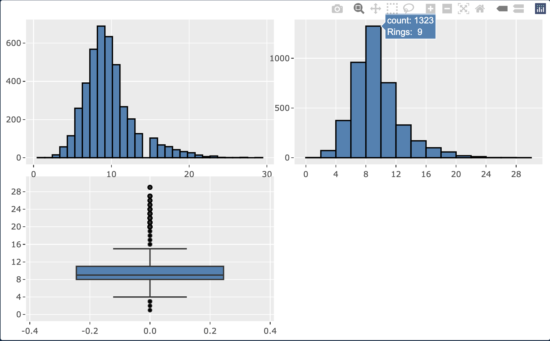
# Create a histogram with the default bin range
p1 <- abalone %>%
  ggplot(aes(x=Rings)) +
  geom_histogram(color="black", fill="steelblue")

# Convert to plotly
p1 <- ggplotly(p1)

# Create a histogram with a custom bin range
p2 <- abalone %>%
  ggplot(aes(x=Rings)) +
  geom_histogram(binwidth = 2, boundary = 0, color="black", fill="steelblue") +
  scale_x_continuous(breaks = seq(0, 30, 4), limits = c(0, 30))

# Convert to plotly
p2 <- ggplotly(p2)

# Create a boxplot
p3 <- abalone %>%
  ggplot(aes(y=Rings)) +
  geom_boxplot(fill="steelblue") +
  scale_y_continuous(breaks = seq(0, 30, 4), limits = c(0, 30))

# Convert to plotly
p3 <- ggplotly(p3)

# Print the plots using the `subplot` function from plotly
p4 <- subplot( p1, p2, p3, nrows = 2 )

p4

# Compute the correlation matrix
corr_matrix <- cor( abalone %>% select(where(is.numeric)), method = "spearman" )

# Convert the correlation matrix into a tidy format
corr_df <- as.data.frame( corr_matrix ) %>%
  rownames_to_column( "Var1" ) %>%
  reshape2::melt( id.vars = "Var1", variable.name = "Var2", value.name = "Correlation" )

# Create a heatmap with ggplot2
heatmap <- ggplot( corr_df, aes(x = Var1, y = Var2, fill = Correlation) ) +
  geom_tile() +
  geom_text( aes(label = round(Correlation, 2)), size = 4 ) +
  scale_fill_gradient2( low = "blue", high = "red", mid = "white", midpoint = 0 ) +
  theme_minimal() +
  theme( axis.text.x = element_text(angle = 45, hjust = 1) )

# Convert the heatmap to a plotly interactive graphic
heatmap <- ggplotly(heatmap)

heatmap

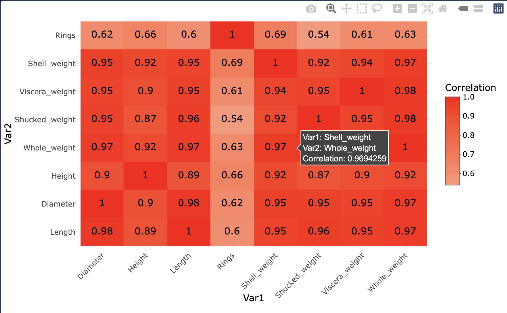
The attributes that are most correlated to Rings are Shell_weight and Height.

RStudio – Data Processing & Plotting with R

Introduction

Further Reading