DataScience Workbook / 08. Data Visualization / 2. Introduction to Scientific Graphing / 2.1 Gnuplot – Creating Plots in the UNIX Shell

Introduction

Gnuplot is a command-line driven graphing utility available for Linux, Windows, and Mac. The tool provides full customization of the graph by specifying values for numerous parameters. When run in a terminal, it allows to change parameter values on the fly and immediately update the graph in the graphical interface, which automatically appears as an additional window. The optimized set of settings can then be copied into a simple bash script that can be run in a loop for multiple files or saved for future reuse. Gnuplot is a simple and robust terminal tool that allows you to quickly generate both 2D and 3D charts.
I recommend this tool for everyday analytical work, where we need to preview analysis results, as well as for generating highly specialized charts of publication quality. Its important advantage is the ability to automatically generate hundreds/thousands of charts of a given type, if needed.

Since version 5.0 and up, there are new features in Gnuplot and enhanced online documentation with a great resource of ready-made demo examples.

Gnuplot Installation

On Linux systems, Gnuplot is usually pre-installed. The other operating systems, including Mac OS and Windows, require quick and straightforward installation. Below, you can find a brief guide that requires you to copy-paste code snippets in the terminal window.

WARNING:
If you don't do NOT know what is terminal or command-line, start with the tutorial(s) that will give you a good introduction:
• TERMINAL, Terminal: the command-line interface
• COMMAND-LINE, Introduction to Unix Shell

on Linux (Debian, Ubuntu)

sudo apt-get update
sudo apt-get install gnuplot

on Mac OS

brew install gnuplot

on Windows and others

Please visit http://www.gnuplot.info/download.html to download the most recent release and follow the instructions provided by RIP Tutorial: Gnuplot Installation or Setup.

Interactive Graphing in the terminal

(on the local machine)

To start a new Gnuplot session, type in the terminal window:

gnuplot

Open Gnuplot in the Terminal
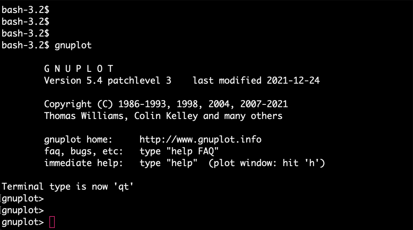
Figure 1. The image shows how to start Gnuplot session in the command-line terminal. When properly activated, Gnuplot displays a welcome message and the prompt changes to ‘gnuplot>’.

Note that the prompt has changed to gnuplot. It means your gnuplot session is launched directly in your terminal window, and you should now enter only gnuplot-compatible syntax instead of Unix commands. For example, the listing directory with ls command is no longer possible.

Open Gnuplot in the Terminal
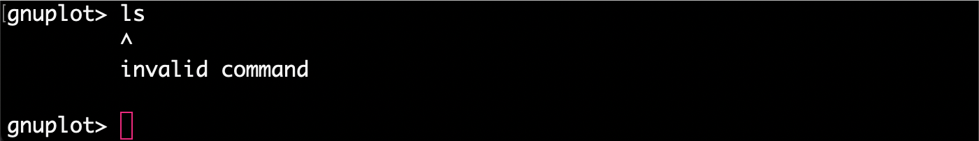
Figure 2. Bash commands are not allowed in the interactive gnuplot session.

However, once you press tab on your keyboard, the list of files available in the current directory will be displayed. This will be useful for copying the file name when graphing data from a file.

Open Gnuplot in the Terminal
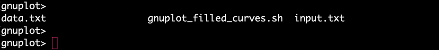
Figure 3. Files in the working disrectory can be displayed by pressing TAB on the keyboard.

Now, let’s plot a simple function, for example sin(x) using default points.
Please, copy-paste the command provided below in the gnuplot-terminal:

plot sin(x) with points

As you noticed, executing the plot command starts the GUI window, which allows an on-the-fly preview of creating graphs and some interactivity with data. You can use the options in the graphical interface to export the chart to a static image in one of the available formats (PDF [vector], SVG [vector], PNG [raster]). In the top menu, there is also an option for adding grid lines and zooming (also possible by selecting the chart area with the mouse). Hovering over any point with the mouse displays its coordinates at the bottom of the GUI window.

Open Gnuplot in the Terminal
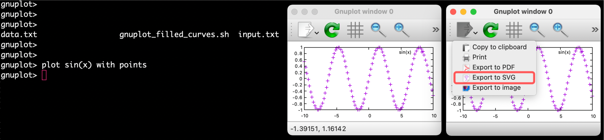
Figure 4. The interactive graph is launched in the separate GUI window which provides options to save image in the selected graphical format.

In the Settings for gnuploting section you will learn the Gnuplot syntax for setting up details of the graph’s layout and plotting commands.

PRO TIP:
The identical syntax of settings can be used directly in the terminal, as well as pasted into a script in Bash. For details, see the next section, Generating static graphs using Bash scripts.
So, it is good practice to create a set of settings in a terminal with a live preview of the graph in a GUI window and then copy-paste those settings into a script. This way, you can easily reuse it in the future or generate the same type of chart in a loop for thousands of samples. That will also allow you to create graphs on a remote machine including HPC infrastructure.

Generating static graphs using Bash scripts

(on the local or remote machine)

In this case, you do NOT have to launch gnuplot session in the terminal. Instead, create an empty file for Bash script, e.g., touch gnuplot_graphing.sh, open the file in any editor, and copy-pased the code snippet provided below. Then save changes.

#!/bin/bash

# BASH VARIABLES
output="simple_graph"
format=png

gnuplot -persist <<- EOF

# LAYOUT SETTINGS
    set terminal '$format'
    set output '$output.$format'

# PLOTTING COMMAND
    plot sin(x) with points

EOF

You can use that snippet as a template for each gnuplotting project and further adjust it by setting up various kinds of plots.

Before we run that script, first, let’s see what’s inside?
At the very top is a shell/kernel syntax #!/bin/bash to let the shell know what type of interpreter to run, and in this example, we ask for Bash. Further, we define 2 variables:

output, which specifies the name of the output image
format, which defines both the format of the image and the selected Gnuplot terminal

Instead of defining variables, you can provide these values directly in the gnuplot section of the script. However, with time you will realize that having those values specified as global variables makes the script more universal and practical for future reuse. Also, this provides the ability to run Gnuplot in a Bash loop to generate the same chart type for multiple inputs.

Finally, there is a gnuplot section, where the <<EOF ... EOF syntax allows to execute the Gnuplot command within a Bash script. All settings contained inside this syntax can be directly pasted from a Gnuplot session run directly in the terminal. In this example, the only exception is using pre-defined variables instead of exact values. To use a Bash variable defined outside the gnuplot section, prefix the variable name with $ and enclose the entire variable in single quotes (for text like variables).

variable --> '$variable'

PRO TIP:
To learn more about Gnuplot variables, loops, and conditional plotting, as well as developing an efficient Bash loop to generate many repetetive charts, see the other tutorial: Gnuplot variables, loops, and conditionals.

The gnuplot section contains two main blocks of commands:

layout settings, where individual components are configured with the set command
Learn more in the section: Graph Layout Settings.
plotting command, where datafile or a selected function is plotted using plot (2D) or splot (3D) commands
Learn more in the section: Plotting Options.

Run the script

To run the script, execute the following command in the terminal window:

. ./gnuplot_graphing.sh

As a result, the simple_graph.png should appear in your working directory.

Gnuplot siple graph
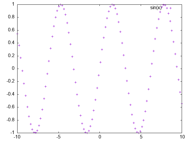
Figure 5. The image shows sin(x) function generated using simple Bash script for gnuplotting.

Congratulations! You have just successfully created your first graph in Gnuplot!

With Gnuplot you can customize literally everything (!) on your chart, including chart title, axis labels, font type and size, margins, legend position, point type and color, background color, and add various additional objects and annotations. You will learn all this in the next section, Graph Layout Settings.

In the following part of this tutorial, you will learn how to customize plotting command and the graph layout settings for your project.

Plotting Options

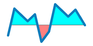
Gnuplot offers graphing of functions (both built-in and user-defined) and custom data loaded from a text file organized into columns. Before we get into the syntax, it is worth mentioning that the program allows you to create 2D and 3D plots, including drawing surfaces. It is also possible to plot multiple traces (data series) on a single chart or to organize multiple charts into subplots.

Gnuplot siple graph
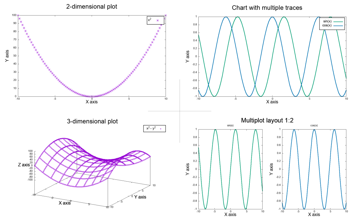
Figure 6. Gnuplot enables graphing in 2D and 3D, and organizing multiple traces within plotting area.

Example dataset

Let us create a simple dataset organized in the 3-column file which we will then use in hands-on exercises of gnuplotting.

File: input.txt

With Gnuplot you can either create graphs:

2D using plot command: plot <arguments>
3D using splot command: splot <arguments>

Both commands can create graphs :

A. using data from an input file structured into columns, e.g., space-separated file: plot 'input.txt' using 1:2
B. using predefined functions, e.g., sin(x), cos(x): plot sin(x)
C. using custom functions, also depending on certain parameters, e.g., f(x) = 0.5 * (x^2 - y^2): splot f(x)

Arguments for Plotting Commands

The syntax and list of arguments for both plot and splot commands are generally the same. The arguments for plotting command are provided in order starting from an optional ranges for X and Y axes defined as an empty square brackets or any of from-to boundary. A value that remains unspecified is automatically assumed from the data. Specifying a graph function is a mandatory argument that either is expressed as y=f(x) mathematical formula or using x:y (x:y:z for 3D) values from input data. The optional use of the title keyword followed by a string in single quotes will name the given trace that will be visible in the legend. The last argument, with, specifies the style of the plotted curve. The user can choose between different data representations, including points with various marker symbols, diverse line types, dots, boxes, filled curves, and more. The overview of available arguments for plotting commands are provided in Table 1.

Table 1. Arguments for Gnuplot plotting commands with examples.

argument	examples	definition	notes
{ranges}	[][] [0:][:10] [pi:pi][0:10]	[x-from:x-to] [y-from:y-to]	optional; first [] for X ranges and second [] for Y ranges; any range or boundary can be empty; empty means automatic adjustment to the data range
[function]	‘input’ using 1:2 sin(x) 0.5 * (x^2 - y^2)	‘filename’ using col-x:col-y or function(x)	required; plot x:y using columns from the input file; plot built-in or customized function(x)
title ‘{string}’	title ‘’ or ti ‘’ ti ‘data serie 1’	title ‘string’	optional; use keyword `title` or `ti` (shortcut) with custom name for plotted trace in the single quotes
with {style}	with points ps 3 with lines lw 2 with linepoints with dots	with {marks type} pointtype {int} pointsize {float} linetype {int} linewidth {float} dots	optional; default: `with l lt 1`; use full argument syntax or shortcuts; for details, see options described in Table 2.

The options of the ‘with’ argument

The with argument enables highly detailed customization of the visualization of the plotted data. There are many styles available that provide the most meaningful representation of your data. Most styles are available for both 2D and 3D graphs, and details are given in Tables 2A and 2B, where the corresponding labels T - true and F - false are given.

Table 2A. The most popular styles for Gnuplot plotting with argument.

name, shortcut	style	type	dash	size	color	colorscale	2D / 3D
lines l	linestyle VAL ls 1	linetype VAL lt 1	dashtype VAL dt 2	linewidth VAL lw 1	linecolor VAL lc 1 lc ‘red’ lc rgb ‘#’	palette `splot` only	T / T
points p	ls VAL	pointtype VAL pt 1	-	pointsize VAL ps 1	lc VAL	palette `splot` only	T / T
linespoints lp	ls VAL	lt VAL pt VAL	dt VAL	lw VAL ps VAL	lc VAL	palette `splot` only	T / T
dots d	ls VAL	lt VAL	-	lw VAL	lc VAL	palette `splot` only	T / T
impulses i	ls VAL	lt VAL	dt VAL	lw VAL	lc VAL	palette `splot` only	T / T

In the first choice, you must decide on the type (shape) of curve plotted from your data. Among the most popular options are lines, points, linespoints (lines with points), dots, and impulses (see Table 2A and Figure 7). These styles have abbreviations from the first letter of the full name that perform the same action. This is hugely convenient for developing draft charts and saves a lot of coding.

Then, with a few additional keywords, you can customize the details of the selected style. In particular you can specify the overall line style, including dashing type, color, tickness; points shape (marker symbol), size, color; and filling style for closed curves (e.g., boxes). For styling options the VAL value is usually determined as an intiger corresponding to a predefined style in a given Gnuplot terminal type (see section Gnuplot Terminal):

linestyle VAL, shortcut: ls , intiger VAL defines line type (solid or dotted line) and its color
linetype VAL, shortcut: lt , intiger VAL assigns a default color for a given line_type
dashtype VAL, shortcut: dt , intiger VAL defines the type of line dashing
linewidth VAL, shortcut: lw , intiger VAL sets the line thickness
linecolor VAL, shortcut: lc , the option changes the default color for a given line_type when the value is an intiger; you can also use common color name, e.g., ‘red’ or additional rgb '#4488bb' syntax
pointtype VAL, shortcut: pt , intiger VAL specifies the shape and color of used points; color encoded by intiger is the same for linetype and pointtype
pointsize VAL, shortcut: ps , intiger VAL sets the size of used points, larger values make points more visible
fillcolor VAL, shortcut: fc , string "red" defines the filling color of filledcurves or boxes
fillstyle VAL, shortcut: fs , syntax <type> float defines the filling type {empty, solid, pattern, palette} and transparency level of filledcurves or boxes
palette, shortcut: pal , the option enables coloring graphs with a colorscale

Gnuplot siple graph
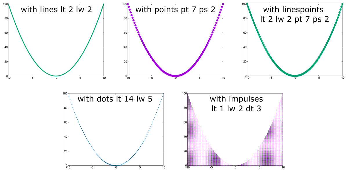
Figure 7. The selected plotting style (lines, points, linespoints, dots, impulses) are adjustable by specifying values of additional params that change line dashing, point shape, color, and size/width. The example shows the y=x^2 function in 2D coordinate space.

Using the styled plotting commands provided in the code block below, you can plot the graphs in Figure 7 yourself.

pl x**2 ti 'with lines lt 2 lw 2' w l lt 2 lw 2                                # lines
pl x**2 ti 'with points pt 7 ps 2' w p pt 7 ps 2                               # points
pl x**2 ti 'with linespoints lt 2 lw 2 pt 7 ps 2' w lp lt 2 lw 2 pt 7 ps 2     # linespoints
pl x**2 ti 'with dots lt 14 lw 5' w d lt 14 lw 5                               # developments
pl x**2 ti 'with impulses lt 1 lw 2 dt 3' w i lt 1 dt 3 lw 2                   # impulses

For those in need, Gnuplot offers many more sophisticated styles, including steps, histogram, filledcurve, boxes, labels, xyerrorbars, vectors, candlesticks, circles, elipses, image, and others.

Table 2B. The other styles for Gnuplot plotting with argument.

name , shortcut	style	type	size	color	colorscale	2D / 3D	fill
steps	ls VAL	lt VAL	lw VAL	lc VAL	-	T / F	-
histogram	ls VAL	lt VAL	lw VAL	lc VAL	-	T / F	-
filledcurve	ls VAL	lt VAL	-	lc VAL	-	T / F	fillstyle {type} VAL fs {empty, solid, pattern, palette} 0.75
boxes	ls VAL	lt VAL	lw VAL	lc VAL	see fill	T / T	fs {type} VAL
labels #	-	-	font ‘Arial, 14’	textcolor VAL tc ‘red’	textcolor palette	T / T	-
vectors #	ls VAL	lt VAL	lw VAL	lc VAL	see fill	T / T	filled head { , palette}
xyerrorbars #	ls VAL	lt VAL	lw VAL	lc VAL	palette	T / T	-
candlesticks #	ls VAL	lt VAL	lw VAL	lc VAL	palette	T / F	-
circles #	ls VAL	lt VAL	lw VAL	lc VAL	palette	T / T	-
…and more

# Plot styles (shapes) marked with # are only for datafiles and requires specifying additional columns for labels (+1 col), xy errors (+2 cols), vectors coordinates (+2 or +3 cols).

Gnuplot siple graph
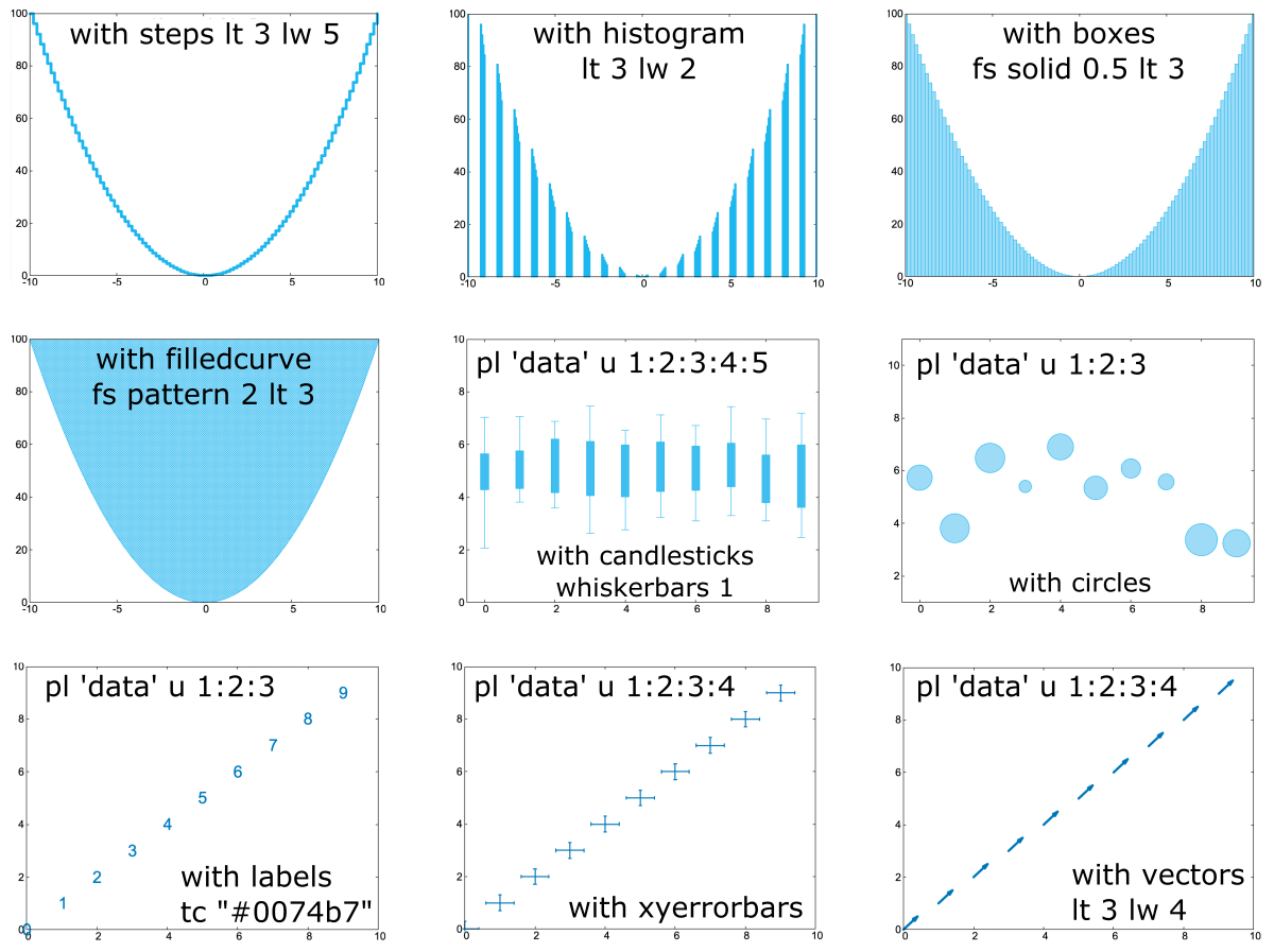
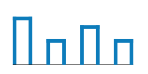
Figure 8. The selected plotting style (steps, histogram, boxes, filledcurves, labels, xyerrorbars, vectors, candlesticks, circles) are adjustable by specifying values of additional params that change color, filling pattern, label font, and size/width. The example shows the y=x^2 function in 2D coordinate space and/or simple x:y input data.

Using the styled plotting commands provided in the code block below, you can plot the graphs in Figure 7 yourself.

GRAPH	command
STEPS	`pl x**2 ti 'with steps' w steps lt 3 lw 5`
HISTOGRAM	`pl x**2 ti 'with histogram' w histogram lt 3 lw 2`
BOXES	`pl x**2 ti 'with boxes' w boxes fs solid 0.5 lt 3`
FILLEDCURVE	`pl x**2 ti 'with filledcurve' w filledcurve fs pattern 2 ls 3`
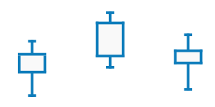
CANDLESTICKS (using 1:2:3:4:5)	`pl 'data.txt' using 1:(5.5+rand(0)):(4-2*rand(0)):(6.5+rand(0)):(4.5-rand(0)-0.1) w candlesticks whiskerbars 1 lc 3`
CIRCLES (using 1:2:3)	`pl [-0.5:9.5][0:10] 'data.txt' using 1:(3+4rand(0)):(0.5sqrt(rand(0))) ti 'with circles' w circles lt 3`
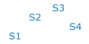
LABELS (using 1:2:3)	`pl [0:10][0:10] 'data.txt' u 1:2:3 ti 'with labels' w labels font 'Arial,20' tc '#0074b7'`
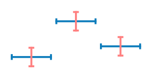
XYERRORBARS (using 1:2:3:4)	`pl [0:10][0:10] 'data.txt' u 1:2:(0.4):(0.3) ti 'with xyerrorbars' w xyerrorbars lt 14 lw 2`
VCECTORS (using 1:2:3:4)	`pl [0:10][0:10] 'data.txt' u 1:2:(0.4):(0.5) ti 'with vectors' w vectors lt 14 lw 4`

2D Plots using plot

Below, you can learn the general syntax for 2D plot command and explore some practical examples.

plot {ranges} [function] title '{string}' with {style}

plot [-pi:pi][] sin(x) title 'Plot sin(x) function' with line linetype 2 linewidth 3

plot [0:][:10] 'input.txt' using 1:2 title 'Plot y=x using data columns' with points pointtype 2 pointsize 3

3D Plots using splot

Below, you can learn the general syntax for 3D splot command and explore some practical examples.

splot {ranges} [function] title '{string}' with {style}

splot [][][] x**2 - y**2 title '3D plot: x^2 - y^2' with points pointtype 6 pointsize 1

splot [0:10][0:10][0:10] 'input.txt' using 1:2:3 title 'Plot x:y:z using data columns' with line linetype 2 linewidth 3

Plot Functions vs. Data from a File

Plot Functions

A. Create graph using predefined functions:

SYNTAX: plot function(x)

plot sin(x)

B. Create grapgh using custom functions, also depending on certain parameters:

SYNTAX: plot function(x)

a = 0.9

# 2D
f(x) = a * x**2
plot f(x)

# 3D
g(x) = a * (x**2 - y**2)
splot g(x)

Plot Custom Data

C. Create graph using data from an input file structured into columns, e.g., space-separated TXT file:

SYNTAX: plot ‘filename’ using col-x:col-y

plot 'input.txt' using 1:2            # 2D
splot 'input.txt' using 1:2:3         # 3D

Specify in order x:y values providing indexes of corresponding columns in the input file. In Gnuplot numbering columns starts with 1. You can provide any column index to feed x or y values. You can also use the same column for both, e.g., using 2:2 or build a custom function using values from column for selected dimension, e.g., using 1:($1**2).

Graph Layout Settings

set syntax

Gnuplot Terminal

Gnuplots provides the opportunity to save graphs in numerous different formats, including popular raster graphics (PNG, JPEG), vector graphics (SVG, PDF), and many more (Latex, DXF, Excl, Corel, X11). More about available terminal types you can learn from Gnuplot Docs and explore some examples via Gnuplotting tutorial.

Use set terminal syntax to determine what kind of output to generate.

set terminal {name} size {x,y} enhanced font '{name, size} '

set terminal pngcairo size 1200,800 enhanced font 'Arial,14'

Gnuplot siple graph
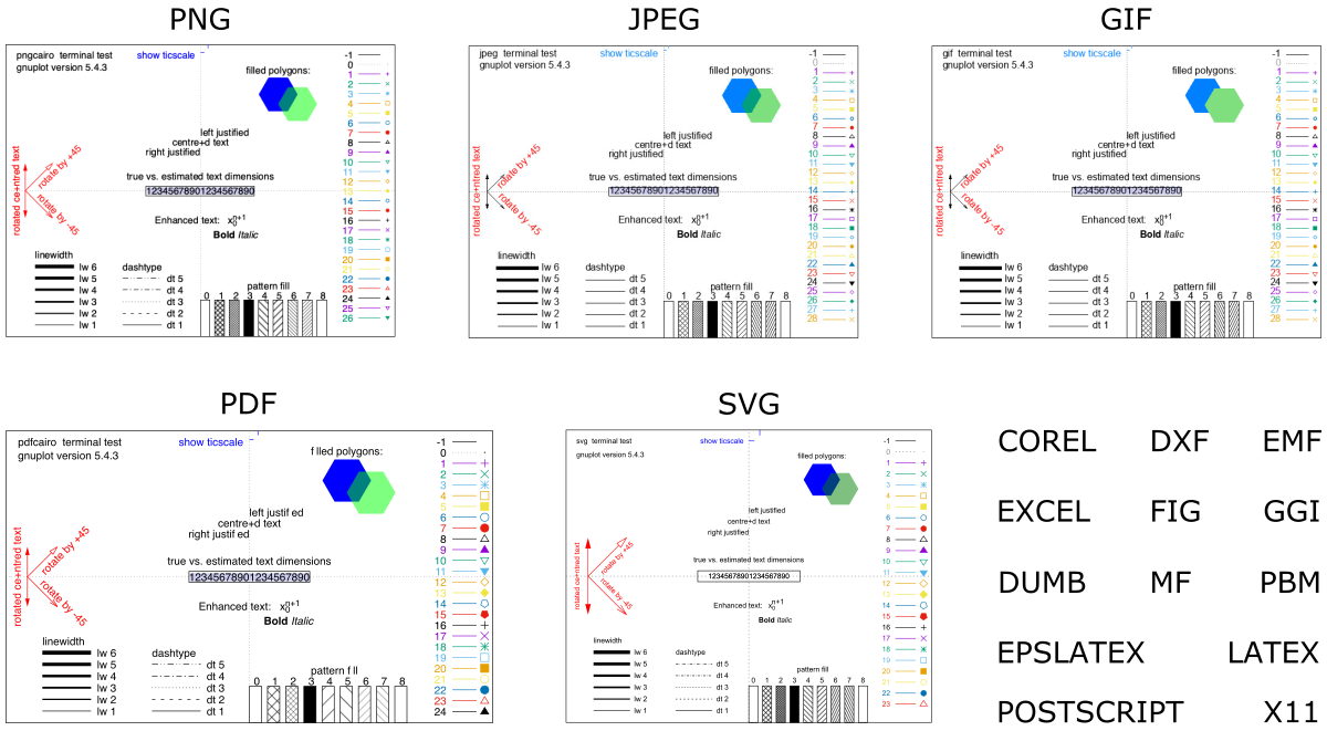
Figure 9. Pre-defined styles for selected Gnuplot terminals (raster: PNG, JPEG, GIF; vector: PDF, SVG). There are many more terminals available in Gnuplot.

Gnuplot: Creating Plots in the UNIX Shell

Aleksandra Badaczewska