
DataScience Workbook / 07. Data Acquisition and Wrangling / 2. Data Manipulation / 2.1 Manipulating Excel Data Sheets / 2.1.4 Merge Two Spreadsheets using a Common Column
Introduction
Excel is most popular among researchers because of its ease of use and tons of useful features. In most cases scripting is the most efficient way to do these simple operations, but practicality of Excel for researchers and the cryptic scripting commands will always make excel a better choice. Most common case of merging 2 spreadsheets is when users have a list of gene ids and another list of geneids with function. To merge these 2 sheets using the gene-ids, we can use the VLOOKUP function.
Data
Typically, users will have something like this:
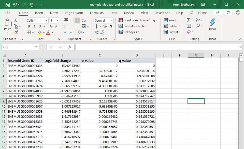
Sheet1 : list of gene ids with differential gene expression results
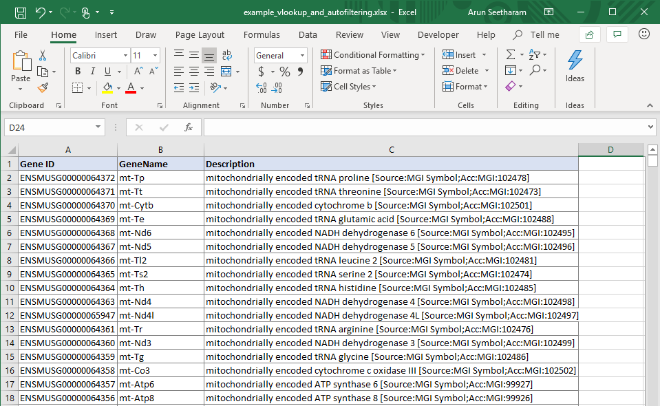
Sheet2: list of gene ids with its annotation information
Now, to add GeneID and GeneName information for the Sheet1 using the information from Sheet2 using Ensembl Gene ID as the common field/column, we can use the VLOOKUP function.
Formula
Type: VLOOKUP on the Sheet1 (E1) cell, you should see typical usage for the command as shown below. It needs 4 pieces of inforamtion:
lookup_value: which cell to use for looking up the value? since we need to look up information forEnsembl Gene IDit should beA2heretable_array: where to look up? the entire table where the annotation is stored. This shoudl be the full table in Sheet2 (in this case:Sheet2!$A$2:$C$49672)col_index_num: what cell value to print for matching ids? Since we need GeneID and it is the 2nd column of Sheet2, we should use the value of2hererange_lookup: do you need an exact match or approximate match? Since each gene id is unique, we need exact match, so we fillFALSEhere
The compelte formula looks like this:
=VLOOKUP(A2,Sheet2!$A$2:$C$49672,2,FALSE)
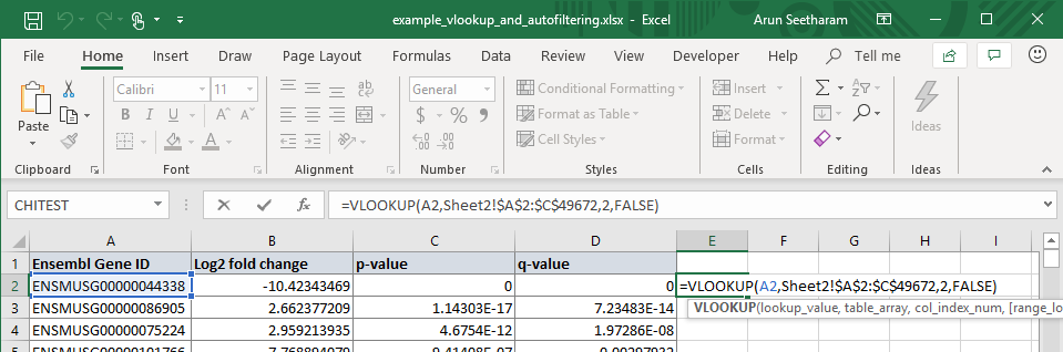
Note the $ for both rows and columns of the table array, this prevetns the excel from incrementing when the formula is dragged to other cells. This is because we want to keep out table_array fixed, regardless where we use the formula in the Sheet1
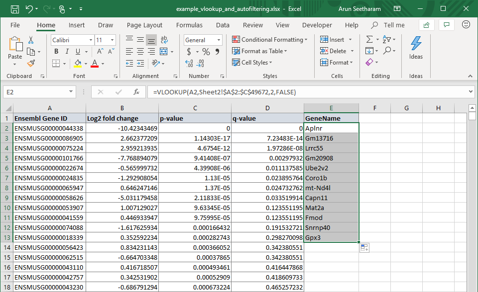
Next, we need to drag this formula down using the + sign that appears on the lower right of the cell containing formula. You can also double click on it to automatically fill the formula for you. It should correctly fill in the GeneID column for you.
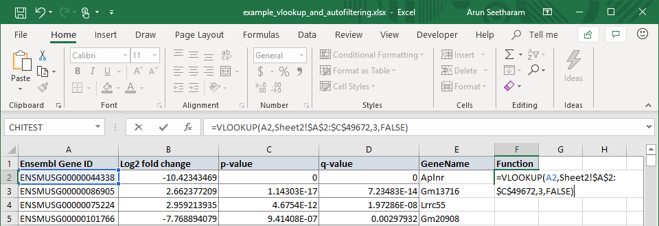
For filling out the GeneName follow the same steps, but instead of using col_index_num value of 2, we will use 3 which is for Description in the Sheet2
=VLOOKUP(A2,Sheet2!$A$2:$C$49672,3,FALSE)
Again, click and drag or double click the + sign that appears on the lower right of the cell to fill all other cells in that column.
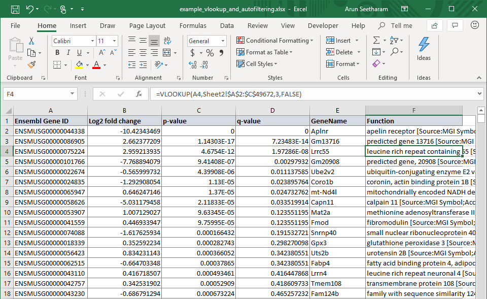
You should now have the complete table with both functions and gene names, now!