
DataScience Workbook / 05. Introduction to Programming / 4. Introduction to R programming / 4.3 tidyverse - R packages set for advanced exploratory data analysis
Introduction
This tutorial is a simplified introduction to:
tidyversepackage- Data download within R
- Data cleaning & wrangling
- Exploratory data analysis
- The goal of EDA is to uncover insights, and check assumptions about the data.
- We achieve this by visualising and applying statistical techniques on the data.
The code below installs a set of R packages. In this case, the code creates a vector called “packages” which only contains the “tidyverse” package name.
Then, the code checks if the “tidyverse” package is already installed by checking if the package name is present in the rownames of the installed.packages() object. The result of this check is stored in the “installed_packages” object.
If the “tidyverse” package is not installed, the code uses the install.packages() function to install the package. If the package is already installed, the code outputs a message indicating that the package is already installed.
The code uses the “any” function to check if there are any uninstalled packages in the “packages” vector, and the “cat” function to print out a message indicating the status of the package installation.
# Package names
packages <- c( "tidyverse" )

# Install uninstalled packages
installed_packages <- packages %in% rownames( installed.packages() )
if ( any(installed_packages == FALSE) ) {
  install.packages( packages[!installed_packages] )
} else {
  cat("The package(s) is/are already installed!\n")
}
## The package(s) is/are already installed!
# Loading packages
invisible( lapply(packages, library, character.only = TRUE) )
## ── Attaching packages ────────────────────────────── tidyverse 1.3.2 ──
## ✔ ggplot2 3.4.1     ✔ purrr   1.0.1
## ✔ tibble  3.1.8     ✔ dplyr   1.1.0
## ✔ tidyr   1.3.0     ✔ stringr 1.5.0
## ✔ readr   2.1.4     ✔ forcats 1.0.0
## ── Conflicts ───────────────────────────────── tidyverse_conflicts() ──
## ✖ dplyr::filter() masks stats::filter()
## ✖ dplyr::lag()    masks stats::lag()
library(tidyverse) will load the core tidyverse packages:
ggplot2, for data visualisation.
dplyr, for data manipulation.
tidyr, for data tidying.
readr, for data import.
purrr, for functional programming.
tibble, for tibbles, a modern re-imagining of data frames.
stringr, for strings.
forcats, for factors.
source.
From the gapminder project, we obtain data for “GDP per capita”, “Life expectancy”, “Population”, and “Country codes”.
url <- "https://github.com/Gapminder/csv-conf-2017-talk/raw/master/data/ddf--bubbles-2/"
file1 <- "ddf--datapoints--gdp_per_capita--by--country--time.csv"
gdp_per_capita <- read_csv( paste0(url, file1) )
## Rows: 43639 Columns: 3
## ── Column specification ───────────────────────────────────────────────
## Delimiter: ","
## chr (1): country
## dbl (2): time, gdp_per_capita
##
## ℹ Use `spec()` to retrieve the full column specification for this data.
## ℹ Specify the column types or set `show_col_types = FALSE` to quiet this message.
gdp_per_capita
## # A tibble: 43,639 × 3
##    country  time gdp_per_capita
##    <chr>   <dbl>          <dbl>
##  1 afg      1800            603
##  2 alb      1800            667
##  3 dza      1800            716
##  4 and      1800           1197
##  5 ago      1800            618
##  6 atg      1800            757
##  7 arg      1800           1507
##  8 arm      1800            514
##  9 abw      1800            833
## 10 aus      1800            815
## # … with 43,629 more rows
file2 <- "ddf--datapoints--life_expectancy--by--country--time.csv"
life_expectancy <- read_csv(paste0(url, file2))
## Rows: 54787 Columns: 3
## ── Column specification ───────────────────────────────────────────────
## Delimiter: ","
## chr (1): country
## dbl (2): time, life_expectancy
##
## ℹ Use `spec()` to retrieve the full column specification for this data.
## ℹ Specify the column types or set `show_col_types = FALSE` to quiet this message.
life_expectancy
## # A tibble: 54,787 × 3
##    country  time life_expectancy
##    <chr>   <dbl>           <dbl>
##  1 afg      1800            28.2
##  2 alb      1800            35.4
##  3 dza      1800            28.8
##  4 and      1800            NA
##  5 ago      1800            27.0
##  6 atg      1800            33.5
##  7 arg      1800            33.2
##  8 arm      1800            34
##  9 abw      1800            34.4
## 10 aus      1800            34.0
## # … with 54,777 more rows
file3 <- "ddf--datapoints--population--by--country--time.csv"
population <- read_csv( paste0(url, file3) )
## Rows: 54787 Columns: 3
## ── Column specification ───────────────────────────────────────────────
## Delimiter: ","
## chr (1): country
## dbl (2): time, population
##
## ℹ Use `spec()` to retrieve the full column specification for this data.
## ℹ Specify the column types or set `show_col_types = FALSE` to quiet this message.
population
## # A tibble: 54,787 × 3
##    country  time population
##    <chr>   <dbl>      <dbl>
##  1 afg      1800    3280000
##  2 alb      1800     410445
##  3 dza      1800    2503218
##  4 and      1800       2654
##  5 ago      1800    1567028
##  6 atg      1800      37000
##  7 arg      1800     534000
##  8 arm      1800     413326
##  9 abw      1800      19286
## 10 aus      1800     351014
## # … with 54,777 more rows
After reading the country_code in, the function “str_to_title” is used to convert all the values in the “world_4region” column to title case. In other words, it capitalizes the first letter of each word in the column.
file4 <- "ddf--entities--country.csv"
country_code <- read_csv( paste0(url, file4) )
## Rows: 273 Columns: 5
## ── Column specification ───────────────────────────────────────────────
## Delimiter: ","
## chr (3): country, name, world_4region
## dbl (2): latitude, longitude
##
## ℹ Use `spec()` to retrieve the full column specification for this data.
## ℹ Specify the column types or set `show_col_types = FALSE` to quiet this message.
country_code$world_4region <- str_to_title( country_code$world_4region )
country_code
## # A tibble: 273 × 5
##    country   name                  world_4region latitude longitude
##    <chr>     <chr>                 <chr>            <dbl>     <dbl>
##  1 abkh      Abkhazia              Europe            NA       NA
##  2 afg       Afghanistan           Asia              33       66
##  3 akr_a_dhe Akrotiri and Dhekelia Europe            NA       NA
##  4 ala       Åland                 Europe            60.2     20
##  5 alb       Albania               Europe            41       20
##  6 dza       Algeria               Africa            28        3
##  7 asm       American Samoa        Asia             -11.1   -171.
##  8 and       Andorra               Europe            42.5      1.52
##  9 ago       Angola                Africa           -12.5     18.5
## 10 aia       Anguilla              Americas          18.2    -63.0
## # … with 263 more rows
Combining the different tibbles and removing missing data.
country_code %>%
  left_join( life_expectancy ) %>%
  left_join( gdp_per_capita ) %>%
  left_join( population ) %>%
  select( name:population ) %>%
  rename_at( vars(name, world_4region, time), ~ c("country", "continent", "year") ) %>%
  drop_na() %>%
  mutate( year = as.Date(paste(year, "-01-01", sep = "", format = "%Y-%b-%d"))) -> gapminder_df
## Joining with `by = join_by(country)`
## Warning in left_join(., life_expectancy): Each row in `x` is expected to match at most 1 row in `y`.
## ℹ Row 2 of `x` matches multiple rows.
## ℹ If multiple matches are expected, set `multiple = "all"` to silence
##   this warning.
## Joining with `by = join_by(country, time)`
## Joining with `by = join_by(country, time)`
gapminder_df
## # A tibble: 41,124 × 8
## country conti…¹ latit…² longi…³ year life_…⁴ gdp_p…⁵ popul…⁶
## <chr> <chr> <dbl> <dbl> <date> <dbl> <dbl> <dbl>
## 1 Afghanis… Asia 33 66 1800-01-01 28.2 603 3280000
## 2 Afghanis… Asia 33 66 1801-01-01 28.2 603 3280000
## 3 Afghanis… Asia 33 66 1802-01-01 28.2 603 3280000
## 4 Afghanis… Asia 33 66 1803-01-01 28.2 603 3280000
## 5 Afghanis… Asia 33 66 1804-01-01 28.2 603 3280000
## 6 Afghanis… Asia 33 66 1805-01-01 28.2 603 3280000
## 7 Afghanis… Asia 33 66 1806-01-01 28.2 603 3280000
## 8 Afghanis… Asia 33 66 1807-01-01 28.1 603 3280000
## 9 Afghanis… Asia 33 66 1808-01-01 28.1 603 3280000
## 10 Afghanis… Asia 33 66 1809-01-01 28.1 603 3280000
## # … with 41,114 more rows, and abbreviated variable names ¹continent,
## # ²latitude, ³longitude, ⁴life_expectancy, ⁵gdp_per_capita,
## # ⁶population
Checking data for the different continents. Here, Australia is categorised under Asia.
gapminder_df %>%
  distinct( continent )
## # A tibble: 4 × 1
##   continent
##   <chr>
## 1 Asia
## 2 Europe
## 3 Africa
## 4 Americas
gapminder_df %>% filter( grepl("[aA]ustralia", country) )
## # A tibble: 216 × 8
## country conti…¹ latit…² longi…³ year life_…⁴ gdp_p…⁵ popul…⁶
## <chr> <chr> <dbl> <dbl> <date> <dbl> <dbl> <dbl>
## 1 Australia Asia -25 135 1800-01-01 34.0 815 351014
## 2 Australia Asia -25 135 1801-01-01 34.0 816 350143
## 3 Australia Asia -25 135 1802-01-01 34.0 818 349274
## 4 Australia Asia -25 135 1803-01-01 34.0 820 348407
## 5 Australia Asia -25 135 1804-01-01 34.0 822 347543
## 6 Australia Asia -25 135 1805-01-01 34.0 824 346681
## 7 Australia Asia -25 135 1806-01-01 34.0 826 345821
## 8 Australia Asia -25 135 1807-01-01 34.0 828 344963
## 9 Australia Asia -25 135 1808-01-01 34.0 830 344107
## 10 Australia Asia -25 135 1809-01-01 34.0 832 343253
## # … with 206 more rows, and abbreviated variable names ¹continent,
## # ²latitude, ³longitude, ⁴life_expectancy, ⁵gdp_per_capita,
## # ⁶population
Reading in list of countries that are part of Oceania.
oceania <- read.csv( "oceania.csv", header = T ) # wikipedia
oceania
##                                V1
## 1                       Australia
## 2                     New Zealand
## 3                            Fiji
## 4                Papua New Guinea
## 5                 Solomon Islands
## 6                         Vanuatu
## 7  Federated States of Micronesia
## 8                        Kiribati
## 9                Marshall Islands
## 10                          Nauru
## 11                          Palau
## 12                          Samoa
## 13                          Tonga
## 14                         Tuvalu
sum( oceania$V1 %in% gapminder_df$country )
## [1] 10
In the code below,the “if_else” function is used to check if the values in the “country” column are present in the “V1” column of the “oceania” data frame. If the values are present, the “continent” column is updated with the value “Oceania”. If not, the original value in the “continent” column is kept unchanged.
gapminder_df %>%
  mutate( continent = if_else(country %in% oceania$V1, "Oceania", continent) ) -> gapminder_df

gapminder_df %>% filter( grepl("[aA]ustralia", country) )
## # A tibble: 216 × 8
## country conti…¹ latit…² longi…³ year life_…⁴ gdp_p…⁵ popul…⁶
## <chr> <chr> <dbl> <dbl> <date> <dbl> <dbl> <dbl>
## 1 Australia Oceania -25 135 1800-01-01 34.0 815 351014
## 2 Australia Oceania -25 135 1801-01-01 34.0 816 350143
## 3 Australia Oceania -25 135 1802-01-01 34.0 818 349274
## 4 Australia Oceania -25 135 1803-01-01 34.0 820 348407
## 5 Australia Oceania -25 135 1804-01-01 34.0 822 347543
## 6 Australia Oceania -25 135 1805-01-01 34.0 824 346681
## 7 Australia Oceania -25 135 1806-01-01 34.0 826 345821
## 8 Australia Oceania -25 135 1807-01-01 34.0 828 344963
## 9 Australia Oceania -25 135 1808-01-01 34.0 830 344107
## 10 Australia Oceania -25 135 1809-01-01 34.0 832 343253
## # … with 206 more rows, and abbreviated variable names ¹continent,
## # ²latitude, ³longitude, ⁴life_expectancy, ⁵gdp_per_capita,
## # ⁶population
gapminder_df %>%
  distinct( continent )
## # A tibble: 5 × 1
##   continent
##   <chr>
## 1 Asia
## 2 Europe
## 3 Africa
## 4 Americas
## 5 Oceania
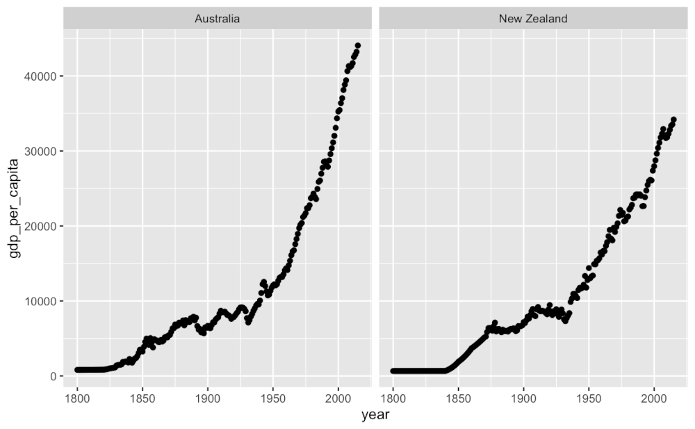
gapminder_df %>%
  filter( country == "New Zealand" | country == "Australia" ) %>%
  # filter( continent == "Oceania" ) %>%
  ggplot( aes(x = year, y = gdp_per_capita) ) +
  geom_point() +
  facet_wrap( . ~ country )
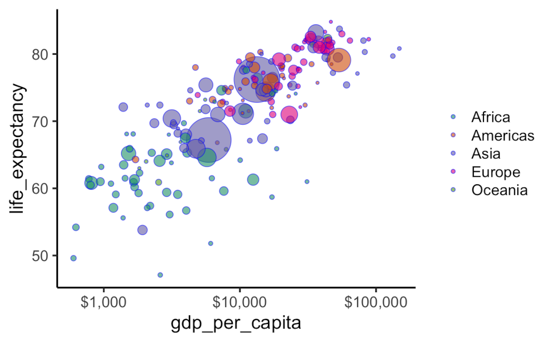
Life expectancy vs GDP Per Capita plot
gapminder_df %>%
  filter( year == "2015-01-01" ) %>%
  ggplot( aes(x = gdp_per_capita, y = life_expectancy) ) +
  scale_x_log10(labels = scales::dollar) +
  geom_point(aes(size = population, fill = continent), shape = 21, colour = "blue", alpha = 0.6) +
  scale_fill_brewer(palette = "Dark2") +
  scale_size_continuous(range = c(1, 20)) +
  guides(size = "none") +
  theme_classic( base_size = 18 ) +
  theme(panel.grid.major.x = element_blank(),
        legend.position = "right",
        legend.title = element_blank())
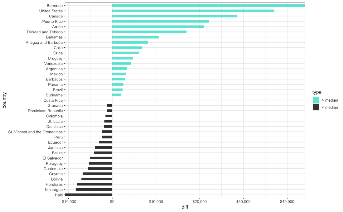
Difference in GDP per Capita for Countries in the Americas in 2015
gapminder_df %>%
  filter(year == "2010-01-01" & continent == "Americas") %>%
  mutate(median = median(gdp_per_capita),
         diff = gdp_per_capita - median,
         type = ifelse(gdp_per_capita < median, "Lower", "Higher")) %>%
  arrange(diff) %>%
  mutate(country = factor(country, levels = country)) %>%
  ggplot( aes(x = country, y = diff, label = country) ) +
  geom_col(aes(fill = type), width = 0.5, alpha = 0.8 )  +
  scale_y_continuous(expand = c(0, 0),
                     labels = scales::dollar) +
  scale_fill_manual(labels = c("> median", "< median"),
                    values = c("Higher" = "Turquoise", "Lower" = "black")) +
  coord_flip() +
  theme_bw( base_size = 12 )
sessionInfo()
## R version 4.2.1 (2022-06-23)
## Platform: x86_64-apple-darwin17.0 (64-bit)
## Running under: macOS Big Sur 11.7.3
##
## Matrix products: default
## LAPACK: /Library/Frameworks/R.framework/Versions/4.2/Resources/lib/libRlapack.dylib
##
## locale:
## [1] en_US.UTF-8/en_US.UTF-8/en_US.UTF-8/C/en_US.UTF-8/en_US.UTF-8
##
## attached base packages:
## [1] stats     graphics  grDevices utils     datasets  methods
## [7] base
##
## other attached packages:
## [1] forcats_1.0.0   stringr_1.5.0   dplyr_1.1.0     purrr_1.0.1
## [5] readr_2.1.4     tidyr_1.3.0     tibble_3.1.8    ggplot2_3.4.1
## [9] tidyverse_1.3.2
##
## loaded via a namespace (and not attached):
##  [1] lubridate_1.9.2     assertthat_0.2.1    digest_0.6.31
##  [4] utf8_1.2.3          R6_2.5.1            cellranger_1.1.0
##  [7] backports_1.4.1     reprex_2.0.2        evaluate_0.20
## [10] highr_0.10          httr_1.4.4          pillar_1.8.1
## [13] rlang_1.0.6         googlesheets4_1.0.1 curl_5.0.0
## [16] readxl_1.4.2        rstudioapi_0.14     rmarkdown_2.21
## [19] labeling_0.4.2      googledrive_2.0.0   bit_4.0.5
## [22] munsell_0.5.0       broom_1.0.3         compiler_4.2.1
## [25] modelr_0.1.10       xfun_0.38           pkgconfig_2.0.3
## [28] htmltools_0.5.4     tidyselect_1.2.0    fansi_1.0.4
## [31] crayon_1.5.2        tzdb_0.3.0          dbplyr_2.3.0
## [34] withr_2.5.0         grid_4.2.1          jsonlite_1.8.4
## [37] gtable_0.3.1        lifecycle_1.0.3     DBI_1.1.3
## [40] magrittr_2.0.3      formatR_1.14        scales_1.2.1
## [43] cli_3.6.0           stringi_1.7.12      vroom_1.6.1
## [46] farver_2.1.1        fs_1.6.1            xml2_1.3.3
## [49] ellipsis_0.3.2      generics_0.1.3      vctrs_0.5.2
## [52] RColorBrewer_1.1-3  tools_4.2.1         bit64_4.0.5
## [55] glue_1.6.2          markdown_1.5        hms_1.1.2
## [58] parallel_4.2.1      fastmap_1.1.0       yaml_2.3.7
## [61] timechange_0.2.0    colorspace_2.1-0    gargle_1.3.0
## [64] rvest_1.0.3         knitr_1.42          haven_2.5.1
Further Reading
- 5. Introduction to Julia programming language
- 5.1 Julia setup: installation, environments and Jupyter integration