DataScience Workbook / 05. Introduction to Programming / 4. Introduction to R programming / 4.2 ggplot2 - R package for customizable graphs and charts
Introduction
ggplot2 is “A system for ‘declaratively’ creating graphics, based on
The Grammar of Graphics. You provide the data, tell ‘ggplot2’ how to map
variables to aesthetics, what graphical primitives to use, and it takes care of
the details.”
The Grammar of Graphics, written by Leland Wilkinson, presents a theoretical
foundation for producing quantitative graphics. The Book
This book is the foundation for ggplot2 created by Hadley Wickham.
We are going to use the faithful and iris data sets to explore ggplot2. The data sets are
part of the R package.
The following are important while using ggplot2.
- Data
- Most important aspect
- Data representation holds the key to what can be done with the data
- Mapping
- Aesthetic mapping Variables in the data linked to graphical properties
- Facet mapping Variables are linked to panels
- Geometries
- geom_*()
- Themes
- Scale
Installing and loading the package.
# install.packages("ggplot2")
library(ggplot2)
Within the code chunk the first line is a comment and it tells the user to install the ggplot2 package. This line is commented out because the package ggplot2 is already installed. The second line loads the ggplot2 package into the current R session. The various functions in the package are now available for use.
The faithful data set contains information on the eruption pattern of the
Old Faithful geyser in Yellowstone National Park.
# Look at the data
str(faithful)
The faithful data set is then examined by displaying its structure with the str() function. This will show the names and types of the variables in the data set.
## 'data.frame':	272 obs. of  2 variables:
##  $ eruptions: num  3.6 1.8 3.33 2.28 4.53 ...
##  $ waiting  : num  79 54 74 62 85 55 88 85 51 85 ...
head(faithful)
##   eruptions waiting
## 1     3.600      79
## 2     1.800      54
## 3     3.333      74
## 4     2.283      62
## 5     4.533      85
## 6     2.883      55
- Data
#data("faithful")
ggplot(data = faithful)

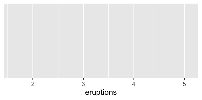
- Mapping
# Adding the mapping
ggplot(data = faithful, mapping = aes(x = eruptions))
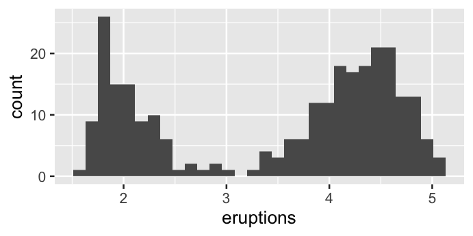
- Geometry
# Basic histogram
ggplot(data = faithful, mapping = aes(x = eruptions)) +
  geom_histogram()
## `stat_bin()` using `bins = 30`. Pick better value with `binwidth`.
The data and the aesthetics can be specified within the layer as well.
ggplot() +
  geom_histogram(data = faithful, aes(x = eruptions))
## `stat_bin()` using `bins = 30`. Pick better value with `binwidth`.

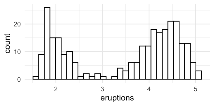
- Theme
ggplot(faithful, aes(x = eruptions)) +
  geom_histogram(colour = "black", fill = "white") +
  # theme_classic()
  # theme_bw()
  theme_minimal()
## `stat_bin()` using `bins = 30`. Pick better value with `binwidth`.
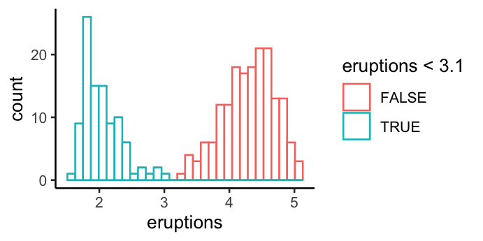
Colour based on mapping
ggplot(faithful, aes(x = eruptions)) +
  geom_histogram(aes(colour = eruptions < 3.1), fill = "white") +
  theme_classic()
## `stat_bin()` using `bins = 30`. Pick better value with `binwidth`.
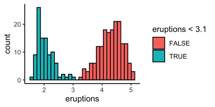
Fill based on mapping
ggplot(faithful, aes(x = eruptions)) +
  geom_histogram(aes(fill = eruptions < 3.1), colour = "black") +
  theme_classic()
## `stat_bin()` using `bins = 30`. Pick better value with `binwidth`.
 Let us now use the
 iris data set for futher exploration of the ggplot2 package.
str(iris)
## 'data.frame':	150 obs. of  5 variables:
##  $ Sepal.Length: num  5.1 4.9 4.7 4.6 5 5.4 4.6 5 4.4 4.9 ...
##  $ Sepal.Width : num  3.5 3 3.2 3.1 3.6 3.9 3.4 3.4 2.9 3.1 ...
##  $ Petal.Length: num  1.4 1.4 1.3 1.5 1.4 1.7 1.4 1.5 1.4 1.5 ...
##  $ Petal.Width : num  0.2 0.2 0.2 0.2 0.2 0.4 0.3 0.2 0.2 0.1 ...
##  $ Species     : Factor w/ 3 levels "setosa","versicolor",..: 1 1 1 1 1 1 1 1 1 1 ...
unique(levels(iris$Species))
## [1] "setosa" "versicolor" "virginica"
head(iris)
##   Sepal.Length Sepal.Width Petal.Length Petal.Width Species
## 1          5.1         3.5          1.4         0.2  setosa
## 2          4.9         3.0          1.4         0.2  setosa
## 3          4.7         3.2          1.3         0.2  setosa
## 4          4.6         3.1          1.5         0.2  setosa
## 5          5.0         3.6          1.4         0.2  setosa
## 6          5.4         3.9          1.7         0.4  setosa
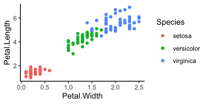
# Basic scatterplot
ggplot(data = iris, mapping = aes(x = Petal.Width, y = Petal.Length)) +
  geom_point(aes(colour = Species))+
  theme_classic()
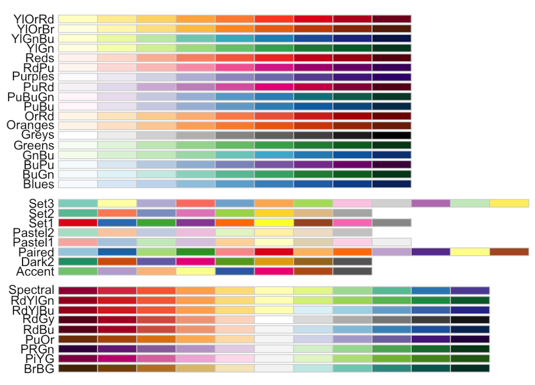
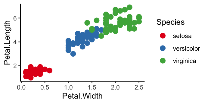
- Scale Adding a different colour scheme
RColorBrewer::display.brewer.all()
ggplot(data = iris, mapping = aes(x = Petal.Width, y = Petal.Length)) +
  geom_point(aes(colour = Species), size = 3) +
  theme_classic() +
  scale_colour_brewer(palette = "Set1")
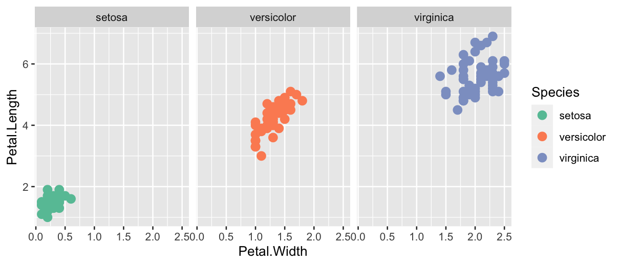
- Facets
ggplot(data = iris, mapping = aes(x = Petal.Width, y = Petal.Length)) +
  geom_point(aes(colour = Species), size = 3) +
  facet_wrap(~ Species) +
  scale_colour_brewer(palette = "Set2")
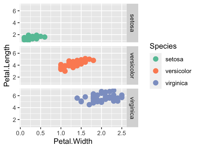
ggplot(data = iris, mapping = aes(x = Petal.Width, y = Petal.Length)) +
  geom_point(aes(colour = Species), size = 3) +
  facet_grid(Species ~ .) +
  scale_colour_brewer(palette = "Set2")
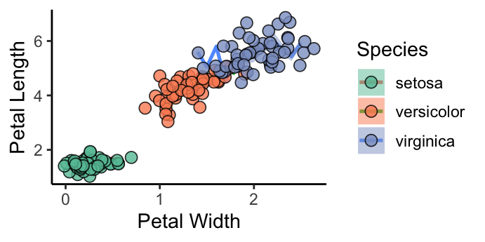
ggplot(iris, aes(x = Petal.Width, y = Petal.Length)) +
  stat_summary(geom = "line", fun = mean, aes(group = Species, colour = Species),
               size = 1) +
  stat_summary(geom = "ribbon", fun.data = mean_se, aes(group = Species, fill = Species),
               alpha = 0.5) +
  # geom_point(aes(fill = Species), size = 3)
  geom_point(aes(fill = Species), position = position_jitter(0.2, seed = 123),
             alpha = 0.8, shape = 21, colour = "black", size = 3) +
  scale_fill_brewer(palette = "Set2") +
  labs( x = "Petal Width", y = "Petal Length") +
  theme_classic(base_size = 12)
sessionInfo()
## R version 4.2.1 (2022-06-23)
## Platform: x86_64-apple-darwin17.0 (64-bit)
## Running under: macOS Big Sur 11.6.7
##
## Matrix products: default
## LAPACK: /Library/Frameworks/R.framework/Versions/4.2/Resources/lib/libRlapack.dylib
##
## locale:
## [1] en_US.UTF-8/en_US.UTF-8/en_US.UTF-8/C/en_US.UTF-8/en_US.UTF-8
##
## attached base packages:
## [1] stats     graphics  grDevices utils     datasets  methods   base
##
## other attached packages:
## [1] ggplot2_3.3.6
##
## loaded via a namespace (and not attached):
##  [1] highr_0.9          pillar_1.8.0       compiler_4.2.1     RColorBrewer_1.1-3
##  [5] tools_4.2.1        digest_0.6.29      evaluate_0.15      lifecycle_1.0.1
##  [9] tibble_3.1.8       gtable_0.3.0       pkgconfig_2.0.3    rlang_1.0.4
## [13] cli_3.3.0          DBI_1.1.3          rstudioapi_0.13    yaml_2.3.5
## [17] xfun_0.31          fastmap_1.1.0      withr_2.5.0        stringr_1.4.0
## [21] dplyr_1.0.9        knitr_1.39         generics_0.1.3     vctrs_0.4.1
## [25] grid_4.2.1         tidyselect_1.1.2   glue_1.6.2         R6_2.5.1
## [29] fansi_1.0.3        rmarkdown_2.14     farver_2.1.1       purrr_0.3.4
## [33] magrittr_2.0.3     scales_1.2.0       htmltools_0.5.3    assertthat_0.2.1
## [37] colorspace_2.0-3   labeling_0.4.2     utf8_1.2.2         stringi_1.7.8
## [41] munsell_0.5.0