DataScience Workbook / 04. Development Environment / 2. Python programming environment(s) / 2.3.3 Jupyter Lab: create an interactive Python notebook
NOTE: Please note that this tutorial requires the user to have a basic understanding of the options available in Jupyter. If you are not familiar with Jupyter, we recommend exploring other tutorials in section 04. Development Environment ⤴ to get started:
- Jupyter: Interactive Web-Based Multi-Kernel DE ⤴
- Getting Started with JupyterLab on a local machine ⤴
- Getting Started with Jupyter Notebook on HPC systems ⤴
Introduction
Jupyter Lab is an interactive web-based tool that allows users to create and share documents that contain live code, equations, visualizations, and narrative text (e.g., documentation), offering benefits such as data exploration, reproducibility, and collaboration.
In Jupyter notebook, users can leverage various Python libraries, including graphical ones, to analyze and visualize data all in one document, providing a powerful and efficient environment for Python-based developments. It offers a convenient way to organize and document a project, making it easier to share and collaborate with others.
Notebooks can be easily shared as a .ipynb file or hosted on online platforms (e.g., Google Colab ⤴), allowing collaborators to access and modify the same document in real-time, which streamlines collaboration and helps to reduce errors and redundancies.
Is Python in Jupyter always good?
YES, Jupyter is a powerful modern interactive development environment!
However, while Python coding in Jupyter offers many advantages, it may not always be the best choice for every project or use case.
✓ Jupyter notebook .ipynb is primarily designed for interactive computing, data exploration, and rapid prototyping, making it an excellent tool for tasks like data analysis, data visualization, and machine learning.
- interactive coding environment that allows you to test code snippets and experiment with different algorithms or techniques
- notebooks make it easy to create visualizations of data using Python libraries like Matplotlib, Seaborn, and Plotly
- notebook format allows you to easily document your code, including adding text, images, or links, which can help with reproducibility and documentation
✗ For small Python scripts, a plain text file script .py is often sufficient and may be more appropriate than a Jupyter notebook .ipynb.
- Plain text files are lightweight, easy to read, and can be executed directly from the command line, which makes them a suitable choice for simple scripts.
- Additionally, plain text files are easier to version control with tools like Git, which can be essential for collaborating and managing code changes.
Learn more from the practical tutorial Text editors: create Python code in terminal text files ⤴.
✗ For production-level Python code, where performance, scalability, and maintainability are critical, other tools may be more suitable. Jupyter notebooks can be challenging to manage with version control systems like Git, which can make it difficult to track changes over time.
✗ For large modular Python developments, IDEs such as Visual Studio Code (VSC) or PyCharm are often a better choice than Jupyter, since they offer more advanced features, like debugging, refactoring, and testing, that are essential for professional development.
Learn more from the practical tutorial PyCharm: IDE for Professional Python Developers ⤴
Python in JupyterLab locally
If you don’t already have Jupyter Lab installed on your local machine, make up for this step by following the instructions in the Installing Jupyter ⤴ section of the Jupyter: Web-Based Programming Interface ⤴ tutorial.
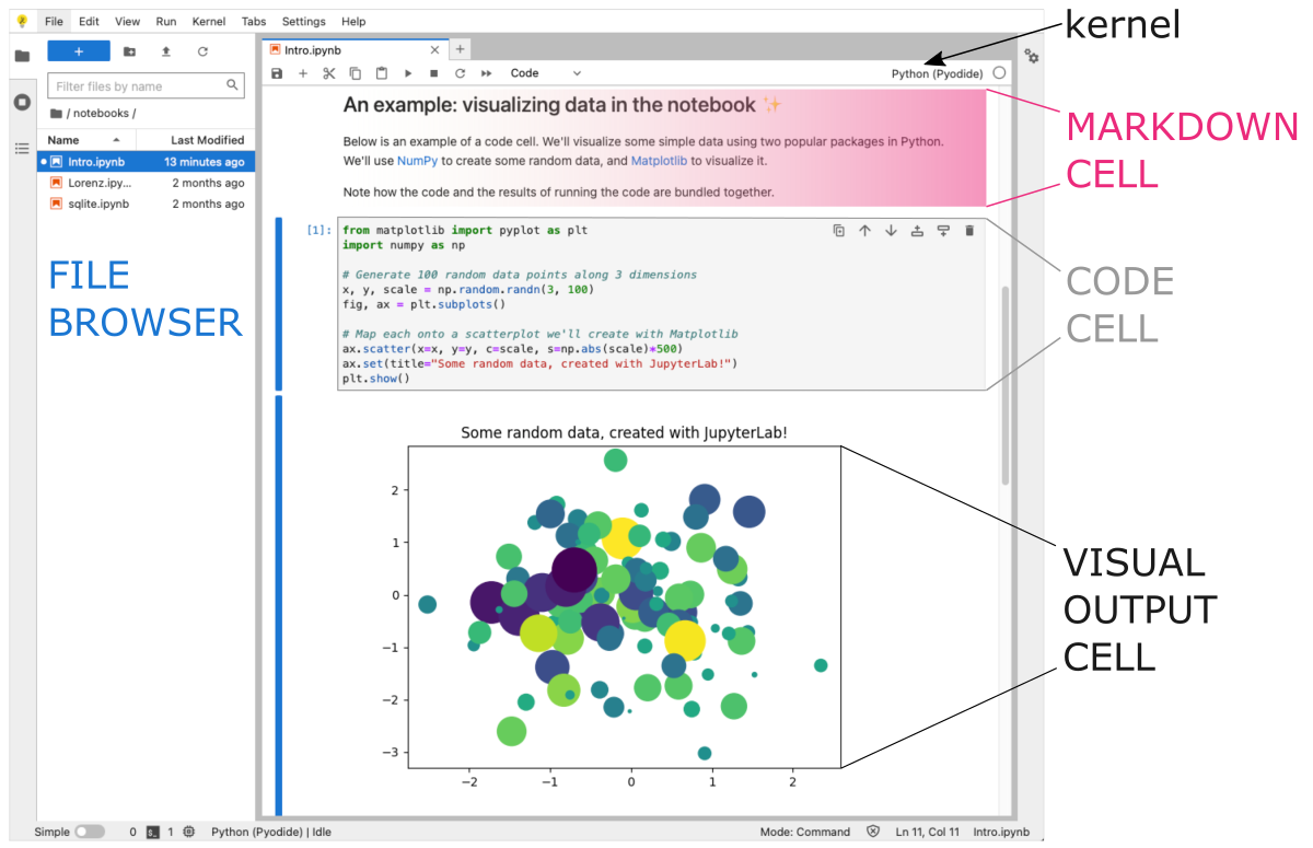
To learn more about Jupyter Lab interface (cell types, opening and saving files, executing the code, and other options) see Getting Started with JupyterLab ⤴ tutorial.
A. Launch Jupyter in the default Python version
The version of Python used in JupyterLab locally depends on the Python kernel that you have installed and selected for your JupyterLab session. So, once you have Jupyter Lab and Python installed on your local machine, you can simply type in the terminal:
jupyter lab
to autmoatically launch the Jupyter Lab interface in your default web browser.
B. Launch Jupyter in the selected Python version
If you want to use a specific version of Python or a specific set of packages, you should create first a new environment with the desired version of Python installed and then activate that environment before you launch JupyterLab interface. For example, to have a kernel with Python in version 3.9 create and activate the Conda environment like that:
conda create -n 'new_env_py3.9' python=3.9
conda activate new_env_py3.9

jupyter lab
You can learn more about creating virtual environments for Python using Conda in the tutorial Python Setup on your computing machine ⤴.
C. Launch Jupyter and switch the Python kernel
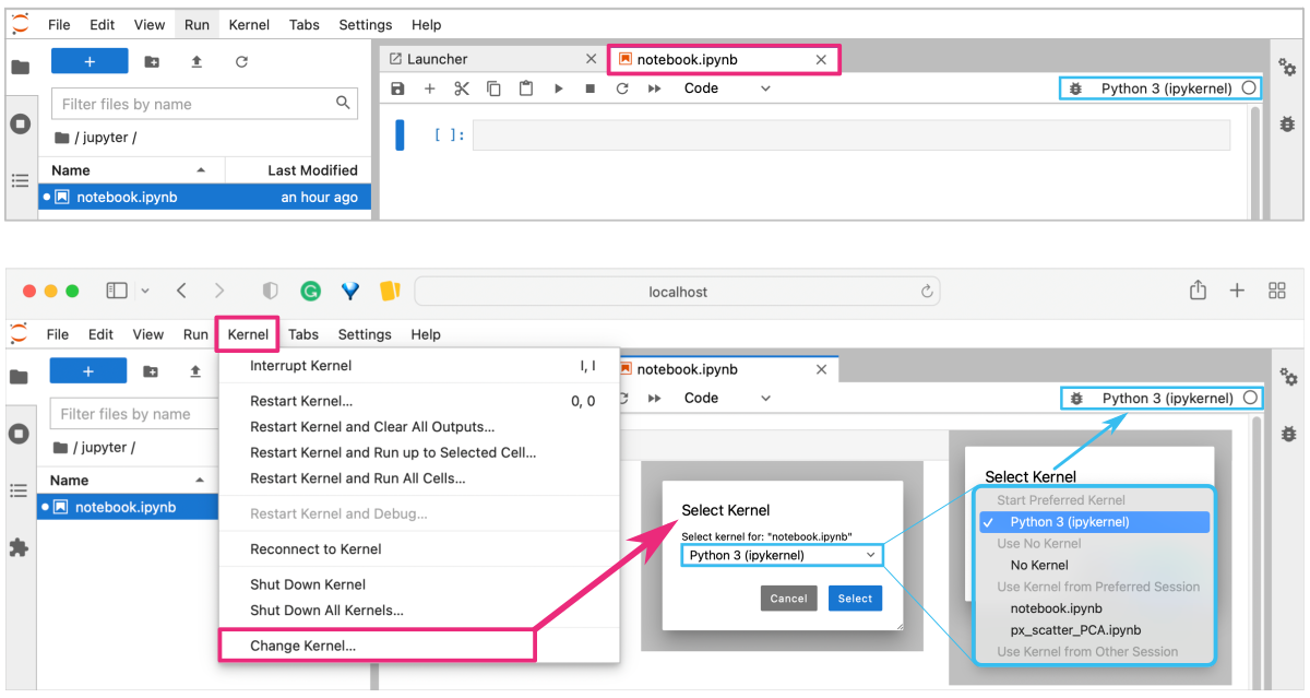
When you create a new notebook in JupyterLab interface, you can select the kernel you want to use for that notebook. If you have multiple kernels installed, you can choose the appropriate kernel for your project.
To check which Python kernel is currently selected, you can click on the kernel name in the top right corner of the notebook interface. This will display a dropdown menu with the currently available kernels. The name of the selected kernel will be highlighted in bold. You can also change the version of Python from the Kernel option in the top menu bar, as shown in the figure below.
Python coding example
- scatterplot by plotly
Example Python-based notebook for creating scatterplot using Plotly.
In this example, we use a simple dataset for a bioinformatics project. Then we will use the pandas library to create a well-structure DataFrame from the input data. Finally, we apply the plotly graphing functions to plot gene expression levels for different samples on a scatterplot.
Pandas ⤴ is a Python data manipulation library that provides data structures for efficiently storing and manipulating large datasets, and tools for cleaning, filtering, and transforming data.
Plotly ⤴ is a Python data visualization library that allows users to create interactive charts and plots that can be easily shared and published online.
1. Install Requirements
Pandas and Plotly are not included in the standard Python library, which means they need to be installed separately if you want to use them in your Python environment. You can install them using pip or conda package managers depending on your preference.
A. Install system-wide with pip (not recommended)
When you install Pandas and Plotly using pip, the libraries are installed system-wide, which means they are available to all Python environments on your machine. This can be beneficial if you want to use these libraries across multiple projects or if you have multiple Python environments that need to access these libraries.
To install Pandas and Plotly using pip, you can run the following commands in your terminal:
pip install pandas
pip install plotly
It's important to note that installing libraries system-wide can also lead to version conflicts and potential compatibility issues with other libraries that you may have installed. It's generally recommended to use virtual environments (e.g., Conda) or containerization tools like Docker to manage your project dependencies and avoid conflicts between different versions of the same library.
Make sure that you have pip installed on your machine before running installation commands.
You can check if pip is installed by running pip --version in your terminal. If pip is not installed, you can download and install it from the official Python website: https://www.python.org/downloads/ ⤴.
B. Install within env with conda (not recommended)
Installing Pandas and Plotly using conda is a better choice in many cases because conda provides a complete package management system that allows you to manage your Python environments and dependencies more easily. It is a more robust and flexible solution than using pip alone.
With Conda, you can create isolated environments for each of your projects, each with its own set of dependencies, which helps to avoid version conflicts and compatibility issues between different libraries. Additionally, conda allows you to install both Python packages and non-Python packages (such as compilers and scientific libraries) from the same command-line interface, making it easier to manage your entire development environment.
Conda can automatically resolve package dependencies and install compatible versions of all required packages, which saves you time and effort in setting up your development environment.
When you install packages using conda, they are installed in the "base" environment by default, which is activated when you start a new terminal session. This means that any packages you install using conda will be available globally, and can potentially lead to version conflicts or compatibility issues with other packages that are already installed on your system.
To avoid these issues, it's recommended that you create a new conda environment for each of your projects, and install the required packages into that environment.
To create a new conda environment, you can use the following command:
conda create --name graphic_env
This will create a new environment called “graphic_env”.
You can then activate the environment using the following command:
conda activate graphic_env
Once activated, any packages you install using conda will be installed only in this environment, and will not affect other environments or the base environment.
To install Pandas and Plotly using conda, you can run the following commands in your terminal:
conda install pandas
conda install plotly
This way, your new project has its own isolated environment with its own set of dependencies.
Now, you are ready to launch Jupyter Lab interface in the activated Conda environment.
[see STEP 2]
The step-by-step guide, provided above, explains how to install new packages into the currently active environment using the conda install command.
You can also specify the packages that you want to install all-in-one step during the environment creation process:
conda create --name graphic_env python=3.9 pandas plotly

conda activate graphic_env
2. Launch Jupyter Lab interface and create a notebook
Once you have all dependencies installed (python=3.9, pandas, plotly) (and activated) on your local machine, launch the Jupyter Lab interface by typing in your terminal:
jupyter Lab
That will open your Jupyter session in a web browser on localhost with a default URL: http://localhost:8889/lab ⤴.
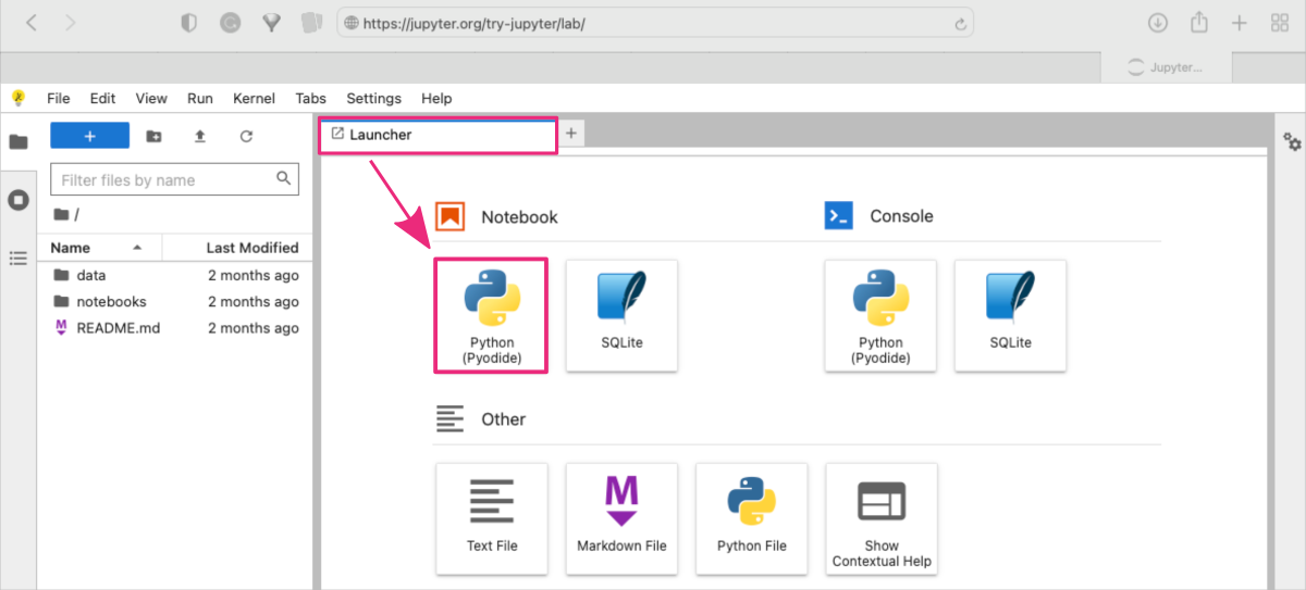
Once the platform has loaded, you can start a new notebook:
- using the Launcher shortcuts by clicking on the Python (Pyodide) button in the Notebook section
or
- using the top menu bar: File : New : Notebook and selecting Python (Pyodide) from the drop-down menu.
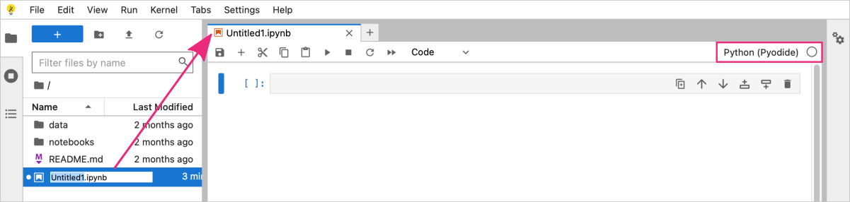
The new notebook should appear as a new tab in your JupyterLab interface.
You can rename the notebook file by double clicking on the filename in the File browser panel on the left-hand side. My notebook is called scatterplot.ipynb.
You can now start writing Python code in the notebook cells and running them by clicking on the Run button in the top menu bar or pressing Shift + Enter to run the current cell and select the cell below it.
3. Python coding example
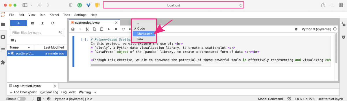
STEP A: Add a markdown cell in the notebook providing the introduction to your project.
You can copy the text provided below and paste it into the first cell in the notebook.
In this project, we will explore the use of:
* `plotly`, a Python data visualization library, to create a scatterplot
* `DataFrame` object of the `pandas` library, to create a structured form of data
*Through this exercise, we aim to showcase the potential of these powerful tools in effectively representing and visualizing complex data sets. By leveraging the capabilities of Plotly and Pandas, we hope to provide insights into the the expression levels of selected genes.*
Now, change the cell type from code to markdown in the top menu bar in the notebook section.
To learn more about Markdown syntax and benefits, check out the practical tutorial Introduction to Markdown ⤴ in Section 09. Project Management : Documentation Improvement Tools ⤴. It will provide you with a hands-on experience of using Markdown to format text, add images, create lists, and more. Don't miss out on this opportunity to enhance your skills!
To execute the cell press Alt + Enter ( use option + return for macOS ).
This will render the markdown content and add a new cell below. By default, new cells are always of the code type.
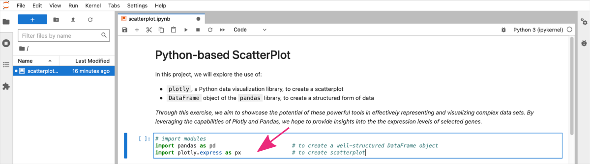
STEP B: Add a code cell to import required modules.
In the next cell add Python code for all required imports, i.e., numpy and matplotlib.
# import modules
import pandas as pd                        # to create a well-structured DataFrame object
import plotly.express as px                # to create scatterplot
To execute the code cell, again press Alt + Enter ( use option + return for macOS ).
STEP C: Add a code cell to load/create input dataset.
In the next code cell add Python code for generating the sample dataset.
Let’s assume we have a CSV file called gene_expression.csv that contains our gene expression data.
Example contents of the input file:
,Gene,Sample,Expression

0,Gene_A,Sample_0,0.018122

1,Gene_B,Sample_0,0.854391

2,Gene_C,Sample_0,0.927634

3,Gene_D,Sample_0,0.086761

4,Gene_E,Sample_0,0.023127

5,Gene_A,Sample_1,0.644789

6,Gene_B,Sample_1,0.713899

7,Gene_C,Sample_1,0.212016

8,Gene_D,Sample_1,0.224403

9,Gene_E,Sample_1,0.111510

10,Gene_A,Sample_2,0.170066

11,Gene_B,Sample_2,0.393153

12,Gene_C,Sample_2,0.312330

13,Gene_D,Sample_2,0.933357

14,Gene_E,Sample_2,0.821238

15,Gene_A,Sample_3,0.422352

16,Gene_B,Sample_3,0.757691

17,Gene_C,Sample_3,0.188810

18,Gene_D,Sample_3,0.894539

19,Gene_E,Sample_3,0.655583

20,Gene_A,Sample_4,0.259517

21,Gene_B,Sample_4,0.592189

22,Gene_C,Sample_4,0.655544

23,Gene_D,Sample_4,0.185386

24,Gene_E,Sample_4,0.716791
This file contains 5 samples and 5 genes. Expression level is a random value between 0 and 1.
We can load this file using Pandas function read_csv(). This assumes that the CSV file is in the same directory as the Jupyter notebook file.
# Load data from the input file in the CSV format
df = pd.read_csv("gene_expression.csv", index_col=0)
df.head()                     # optional: preview the DataFrame structure
Aletrantively, if you do NOT want to load file from a local file system, you can install numpy library, which provides random module. You can use it to generate a sample dataset.
To install a new package from the level of Jupyter notebook, use the !pip command (preceded by an exclamation mark):
!pip install numpy
NOTE: You can call any bash command this way, such as ls to view files.
see the Python code to generate random dataset
Let's create a random dataset of gene expression levels for different samples.
import numpy as np


#1 Generate 2 lists: 'genes' and 'samples' with identifiers for the observations

n = 10

genes = ["Gene_"+str(i) for i in range(n)]

samples = ["Sample_"+str(i) for i in range(n)]


#2 Create the Pandas Dataframe with a random (matrix) dataset matching the size of input lists

df = pd.DataFrame(

        np.random.rand(len(genes), len(samples)),

        columns=samples,

        index=genes

)


df.head()         # optional: preview the DataFrame structure


#3 Rename the index and column names for clarity

df.index.name = "Gene"

df.columns.name = "Sample"


#4 Reset the index to make the gene names a column

df = df.reset_index().melt(id_vars=["Gene"], var_name="Sample", value_name="Expression")
This will create a Pandas DataFrame with 10 samples and 10 genes, where each cell contains a random value between 0 and 1.
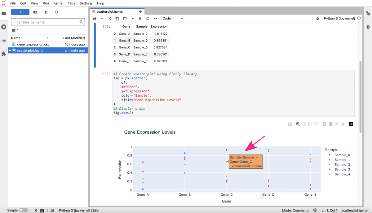
STEP D: Visualizing the Data with Plotly
Now let’s create a scatterplot of the gene expression levels using Plotly:
#1 Create scatterplot using Plotly library
fig = px.scatter(
        df,                                     # DataFrame object storing the data
        x="Gene",                               # column header for the X-axis variable
        y="Expression",                         # column header for the Y-axis values
        color='Sample',                         # column header for the color grouping
        title="Gene Expression Levels"
)

#2 Update graph layout                          # optional section, if you want to customize the plot
fig.update_layout(
    xaxis_title="Genes",
    yaxis_title="Expression",
    legend_title="Sample Index"
)

#3 Display graph
fig.show()
This will create a scatterplot with the gene names on the x-axis, the expression levels on the y-axis, and each sample represented by a different color. Note that Plotly-based graphs are interactive by default. The details about each data point are displayed on the dynamic labels. You can customize their contents, if needed.